Today’s Video tutorial is the one I wish I had access to when I was starting out in OpenCV, in this video I reveal to you some very interesting information about the opencv including great tips regarding when to find the right resources, tutorials for the library.
I’ll start by briefly going over the history of OpenCV and then talk about other exciting topics.
Some of the things I will go through in this video
👉How to navigate the opencv docs to find what you’re looking for. 👉How to get details regarding any OpenCV function. 👉The differences between the C++ and python version of OpenCV and which one you should work with. 👉Pip installation of OpenCV vs Source installation. 👉Where to ask questions regarding OpenCV when you’re stuck.
You can reach out to me personally for a 1 on 1 consultation session in AI/computer vision regarding your project. Our talented team of vision engineers will help you every step of the way. Get on a call with me directlyhere.
Ready to seriously dive into State of the Art AI & Computer Vision? Then Sign up for these premium Courses by Bleed AI
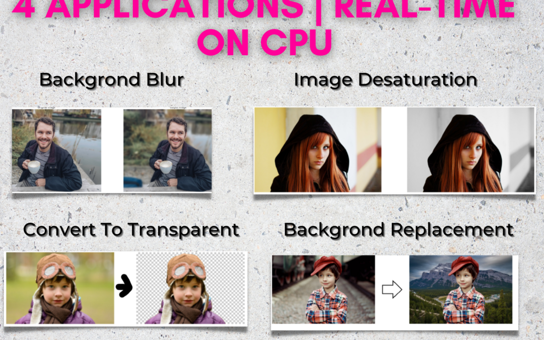
In this tutorial, you’ll learn how to do Real-Time Selfie Segmentation using Mediapipe in Python and then build the following 4 applications.
Background Removal/Replacement
Background Blur
Background Desaturation
Convert Image to Transparent PNG
And not only will these applications work on images but I’ll show you how to apply these to your real-time webcam feed running on a CPU.
Also, the model that we’ll use is almost the same one that Google Hangouts is currently using to segment people, So Yes! We’re going to be learning a State of the Art approach for segmentation.
And on top of that, the code for building all 4 applications will be ridiculously simple.
Interested yet? Then keep reading this full post.
In the first part of this post, we’ll understand the problem of image segmentation and its types, then we’ll understand what selfie segmentation is. After that, we’ll take a look at Mediapipeand how to do selfie segmentation with it. And finally how to build all those 4 applications.
What is Image Segmentation?
If you’re somewhat familiar with computer vision basics then you might be familiar with image segmentation, a very popular problem in Computer Vision.
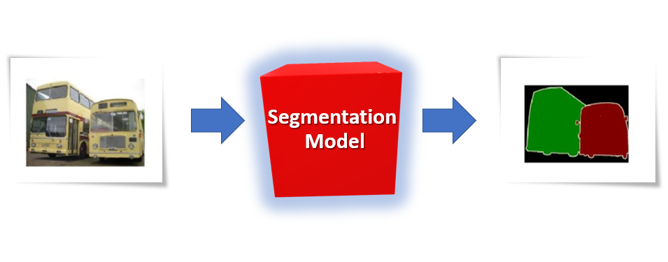
Just like in an object detection task where you localize objects in the image and draw boxes around it, in a segmentation task, you’re almost doing the same thing, but here instead of drawing a bounding box around each object, you’re trying to segment or draw out the exact boundary of each target Object.
Figure 2: A segmentation model is trying to segment out the busses in the image above
In other words, in segmentation, you’re trying to divide the image into groups of pixels based on some specific criteria.
So an image segmentation algorithm will take an input image and output groups of pixels, each group will belong to some class. Normally this output is actually an image mask where each pixel consists of a single number indicating the class it belongs to.
Now the task of image segmentation can be divided into several categories, let’s understand each of them.
Semantic Segmentation.
Instance Segmentation
Panoptic Segmentation
Saliency Detection.
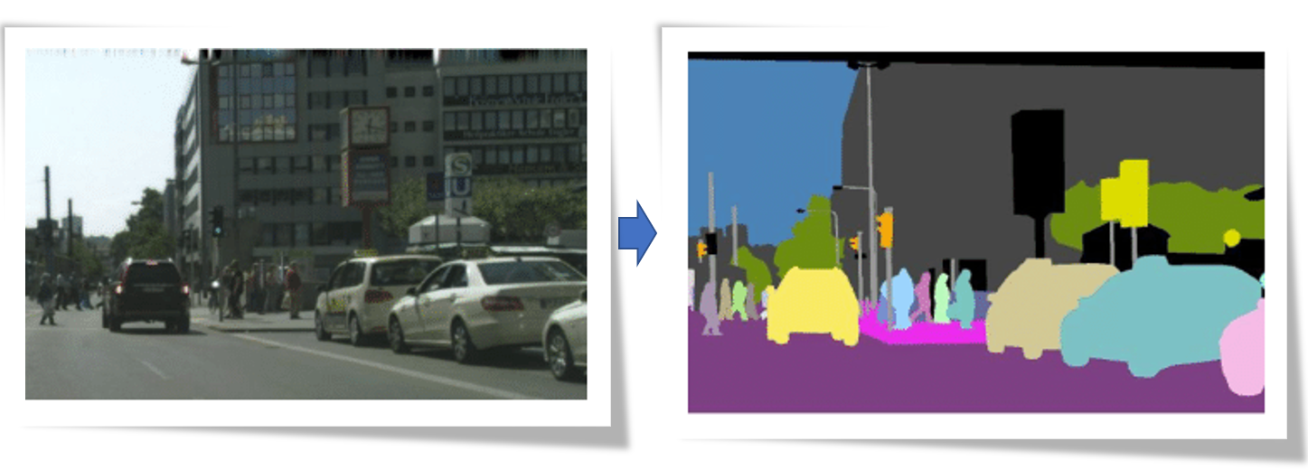
What is Semantic Segmentation?
In this type of segmentation, our task is to assign a class label (pedestrian, car, road, tree etc.) to every pixel in the image.
Figure 3
As you can see all the objects in the image, including the buildings, sky, sidewalk are labeled by a certain color indicating that they belong to a certain class e.g all cars are labeled blue, people are labeled red, and so on.
It’s worth noting that although we can extract any individual class, for e.g. we can say extract all cars by looking for blue pixels but we cannot distinguish between different instances of the same class, for e.g. you can’t reliably say which blue pixel belongs to which car.
What is Instance Segmentation?
Another common category of segmentation is called Instance Segmentation. Here the goal is not to label all pixels in the image but only label some selective classes, for which the model was trained on ( for e.g. cars, pedestrians, etc. ).
Figure 4
As you can see in the image, the algorithm ignored the roads, sky, buildings etc. so here we’re only interested in labeling specific classes.
One other major difference in this approach is that we’re also differentiating between different instances of the same classes i.e. you can tell which pixel belongs to which class and so on.
What is Panoptic Segmentation?
If you’re a curious cat like me, you might wonder, well isn’t there an approach that,
A) Labels all pixels in the image like semantic segmentation.
B) And also differentiates between instances of the same class like instance segmentation.
Well, Yes there is! And it’s called PanopticSegmentation. Where not only every pixel is assigned a class but we can also differentiate between different instances of the same class, i.e. we can tell which pixel belongs to which car.
Figure 5
This type of segmentation is the combination of both instance and semantic segmentation.
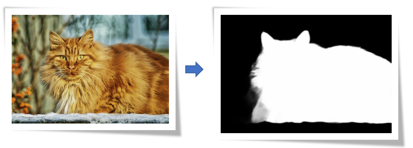
What is Saliency Detection?
Don’t be confused by the word “Detection” here, although Saliency Detection is not generally considered as one of the core segmentation methods but it’s still essentially a major segmentation technique.
So here the goal is to segment out the most salient/prominent (things that stand out ) features in the image.
Figure 6
And this is done regardless of the class of the object. Here’s another example.
Figure 7
As you can see the most obvious object in the above image is the cat, which is exactly what’s being segmented out here.
So in saliency detection where trying to segment out the most standing out features in the image.
Selfie Segmentation:
Alright now that we have understood the fundamental segmentation techniques out there, let’s try to understand what selfie segmentation is.
Figure 8
Well, obviously it’s a no brainer, it’s a segmentation technique that segments out people in images.
Figure 9
You might think, how is this different from semantic or instance Segmentation?
Well, to put it simply, you can consider selfie segmentation as a sort of a mix between semantic segmentation and Saliency detection.
What do I mean by that?
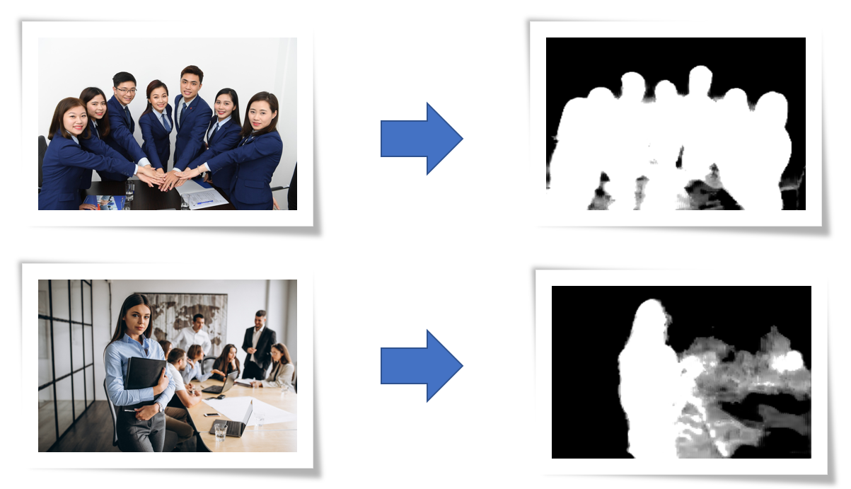
Take a look at the example output of Selfie segmentation on two images below.
Figure 8
In the first image (top) the segmentation is done perfectly, as every person is on a similar scale and prominent in the image, whereas in the second image (bottom) the woman is prominent and is segmented out correctly while her colleagues in the background are not segmented properly.
This is why the technique is called selfie segmentation, it tries to segment out prominent people in the image, ideally everyone to be segmented should be on a similar scale in the image.
This is why I said that this technique is sort of a mix between saliency detection and semantic segmentation.
Now, you might think why do we even need to use another segmentation technique, why not just segment people using semantic or instance segmentation methods.
Well, Actually we could do that. Models like Mask-RCNN, DeepLabv3, and others are really good at segmenting people.
But here’s the problem.
These models although provide State of the Art results but are actually really slow, they aren’t a good fit when it comes to real-time applications especially on CPUs.
This is why the Selfie segmentation model that we’ll use today is specifically designed to segment people and also run at real-time speed on CPU and other low-end hardware. It’s built on a slight modification of the MobielNetv3 model. This model itself contains clever algorithmic innovations for maximum speed and performance gains. To understand more about these algorithmic advances in this model, you can read Google AI’s Blog post on this model.
So what are the use cases for Selfie Segmentation?
The most popular use case for this problem is Video Conferencing. In fact, Google Hangouts is using approximately the same model that we’re going to learn to use today.
Besides Video Conferencing, there are several other use cases for this model that we’re going to explore today.
MediaPipe:
Mediapipe is a cross-platform tool that allows you to run a variety of machine learning models in real-time. It’s designed primarily for facilitating the use of ML in streaming media.
This is the tool that we’ll be using today in order to use the selfie segmentation model. In future tutorials I’ll also be covering the usage of a few other models and make interesting applications out of them. So Stay tuned for those blog posts at Bleed AI.
Alright Now let’s start with the Code!
Selfie Segmentation Code:
[optin-monster slug=”o79lb1j7tdwib0khs6fc”]
To get started with Mediapipe, you first need to run the following command to install it
Now let’s start by importing the required libraries.
import os
import cv2
import numpy as np
import mediapipe as mp
import matplotlib.pyplot as plt
from time import time
Initialize the Selfie Segmentation Model
The first thing that you need to do is initialize the selfie segmentation class using the mp.solutions.selfie_segmentation function and then you need to call the setup function using .SelfieSegmentation(0) now there are two models for segmentation in mediapipe, by passing in 0 you will be using the general model i.e. input is resized to: 256x256x3 (Height, width, columns) and by passing 1 you will be using the landscape model i.e. input resized to: 144x256x3 (Height, width, columns).
You should select the type of model by taking into account the aspect ratio of the original image, although the landscape model is a bit faster. These models automatically resize the input image before passing it through the network and the size of the output image representing the segmentation mask for both models will be the same as the input that is 256x256x1 or 144x256x1.
Now let’s read a sample image using the function cv2.imread() and display the image using the matplotlib library.
# Read an image from the specified path.
sample_img = cv2.imread('media/sample.jpg')

# Specify a size of the figure.
plt.figure(figsize = [10, 10])

# Display the sample image, also convert BGR to RGB for display.
plt.title("Sample Image");plt.axis('off');plt.imshow(sample_img[:,:,::-1]);plt.show()
Application 1: Remove/Replace Background
We will start by learning to use selfie segmentation to change the background of images. But first, we will have to convert the image into RGB format as the MediaPipe library expects the images in this format but the function cv2.imread() reads the images in BGR format and we will use the function cv2.cvtColor() to do this conversion.
Then we will pass the image to the MediaPipe Segmentation function which will perform the segmentation process and will return a probability map with pixel values near 1 for the indexes where the person is located in the image and pixel values near 0 for the background.
# Convert the sample image from BGR to RGB format.
RGB_sample_img = cv2.cvtColor(sample_img, cv2.COLOR_BGR2RGB)

# Perform the segmentation.
result = segment.process(RGB_sample_img)

# Specify a size of the figure.
plt.figure(figsize=[22,22])

# Display the original sample image and the segmentation result with appropriate titles.
plt.subplot(121);plt.imshow(sample_img[:,:,::-1]);plt.title("Original Image");plt.axis('off');
plt.subplot(122);plt.imshow(result.segmentation_mask, cmap='gray');plt.title("Probability Map");plt.axis('off');
Notice that we have some gray areas in the map, this signifies that there are areas where the model was not sure if it was the background or the person. So now what we need to do is do some thresholding and set all pixels above certain confidence to white and all other pixels to black.CodeText
So in this step, we’re going to be thresholding the mask above to get a binary black and white mask with a pixel value 1 for the indexes where the person is located and 0 for the background.CodeText
# Get a binary mask having pixel value 1 for the person and 0 for the background.
# Pixel values greater than the threshold value 0.9 (90% Confidence) will become 1 and the remaining will become 0.
binary_mask = result.segmentation_mask > 0.9


# Display the original sample image and the binary mask with appropriate titles.
plt.figure(figsize=[22,22])
plt.subplot(121);plt.imshow(sample_img[:,:,::-1]);plt.title("Original Image");plt.axis('off');
plt.subplot(122);plt.imshow(binary_mask, cmap='gray');plt.title("Binary Mask");plt.axis('off');
Now we will use the numpy.where() function to create a new image which will have the pixel values from the original sample image at the indexes where the mask image have value 1 (white areas) and replace areas where mask have value 0 (black areas) with 255, to give a white background to the object of the sample image. Right now we’re just adding whtie (255) background but later on we’ll add a separate image as background.
But to create the required output image we will first have to convert the mask image (one channel) into a three-channel image using the function numpy.dstack() as the function numpy.where() will need to have all images to have equal number of channels.
# Stack the same mask three times to make it a three channel image.
binary_mask_3 = np.dstack((binary_mask,binary_mask,binary_mask))

# Create the output image to have white background where ever black is present in the mask.
output_image = np.where(binary_mask_3, sample_img, 255)

# Specify a size of the figure.
plt.figure(figsize=[22,22])

# Display the original sample image and the resultant image.
plt.subplot(121);plt.imshow(sample_img[:,:,::-1]);plt.title("Original Image");plt.axis('off');
plt.subplot(122);plt.imshow(output_image[:,:,::-1]);plt.title("Output Image");plt.axis('off');
Now instead of having a white background if you need to add another background image, you just need to replace 255 with a background image in np.where function
# Read a background image from the specified path.
bg_img = cv2.imread('media/background.jpg')

# Create an output image with the pixel values from the original sample image at the indexes where the mask have
# value 1 and replace the other pixel values (where mask have zero) with the new background image.
output_image = np.where(binary_mask_3, sample_img, bg_img)

# Display the original sample image and the segmentation result
plt.figure(figsize=[22,22])
plt.subplot(131);plt.imshow(sample_img[:,:,::-1]);plt.title("Original Image");plt.axis('off');
plt.subplot(132);plt.imshow(binary_mask, cmap='gray');plt.title("Binary Mask");plt.axis('off');
plt.subplot(133);plt.imshow(output_image[:,:,::-1]);plt.title("Output Image");plt.axis('off');
Create a Background Modification Function
Now we will create a function that will use the selfie segmentation to modify the background of an image depending upon the passed arguments. The followings will be the modifications that the function will be capable of:
Change Background: The function will replace the background of the image with a different provided background image OR it will make the background white for the cases when a separate background image is not provided.
Blur Background: The function will segment out the prominent person and then blur out the background.
Desaturate Background: The function will desaturate (convert to grayscale) the background of the image, giving the image a very interesting effect.
Transparent Background: The function will make the background of the image transparent.
def modifyBackground(image, background_image = 255, blur = 95, threshold = 0.3, display = True, method='changeBackground'):
    '''
    This function will replace, blur, desature or make the background transparent depending upon the passed arguments.
    Args:
        image: The input image with an object whose background is required to modify.
        background_image: The new background image for the object in the input image.
        threshold: A threshold value between 0 and 1 which will be used in creating a binary mask of the input image.
        display: A boolean value that is if true the function displays the original input image and the resultant image
                 and returns nothing.
        method: The method name which is required to modify the background of the input image.
    Returns:
        output_image: The image of the object from the input image with a modified background.
        binary_mask_3: A binary mask of the input image.
    '''

    # Convert the input image from BGR to RGB format.
    RGB_img = cv2.cvtColor(image, cv2.COLOR_BGR2RGB)

    # Perform the segmentation.
    result = segment.process(RGB_img)

    # Get a binary mask having pixel value 1 for the object and 0 for the background.
    # Pixel values greater than the threshold value will become 1 and the remainings will become 0.
    binary_mask = result.segmentation_mask > threshold

    # Stack the same mask three times to make it a three channel image.
    binary_mask_3 = np.dstack((binary_mask,binary_mask,binary_mask))

    if method == 'changeBackground':

        # Resize the background image to become equal to the size of the input image.
        background_image = cv2.resize(background_image, (image.shape[1], image.shape[0]))

        # Create an output image with the pixel values from the original sample image at the indexes where the mask have
        # value 1 and replace the other pixel values (where mask have zero) with the new background image.
        output_image = np.where(binary_mask_3, image, background_image)

    elif method == 'blurBackground':

        # Create a blurred copy of the input image.
        blurred_image = cv2.GaussianBlur(image, (blur, blur), 0)

        # Create an output image with the pixel values from the original sample image at the indexes where the mask have
        # value 1 and replace the other pixel values (where mask have zero) with the new background image.
        output_image = np.where(binary_mask_3, image, blurred_image)

    elif method == 'desatureBackground':

        # Create a gray-scale copy of the input image.
        grayscale = cv2.cvtColor(src = image, code = cv2.COLOR_BGR2GRAY)

        # Stack the same grayscale image three times to make it a three channel image.
        grayscale_3 = np.dstack((grayscale,grayscale,grayscale))

        # Create an output image with the pixel values from the original sample image at the indexes where the mask have
        # value 1 and replace the other pixel values (where mask have zero) with the new background image.
        output_image = np.where(binary_mask_3, image, grayscale_3)

    elif method == 'transparentBackground':

        # Stack the input image and the mask image to get a four channel image.
        # Here the mask image will act as an alpha channel.
        # Also multiply the mask with 255 to convert all the 1s into 255.
        output_image = np.dstack((image, binary_mask * 255))

    else:
        # Display the error message.
        print('Invalid Method')

        # Return
        return

    # Check if the original input image and the resultant image are specified to be displayed.
    if display:

        # Display the original input image and the resultant image.
        plt.figure(figsize=[22,22])
        plt.subplot(121);plt.imshow(image[:,:,::-1]);plt.title("Original Image");plt.axis('off');
        plt.subplot(122);plt.imshow(output_image[:,:,::-1]);plt.title("Output Image");plt.axis('off');

    # Otherwise
    else:

        # Return the output image and the binary mask.
        # Also convert all the 1s in the mask into 255 and the 0s will remain the same.
        # The mask is returned in case you want to troubleshoot.
        return output_image, (binary_mask_3 * 255).astype('uint8')
Now we will utilize the function created above with the argument method='changeBackground' to change the backgrounds of a few sample images and check the results.
# Read a sample image and change background
image2 = cv2.imread('media/sample5.jpg')
modifyBackground(image2, bg_img.copy(), method='changeBackground')
# Read another sample image and a new background and change it.
image3 = cv2.imread('media/sample6.jpg')
bg_img2 = cv2.imread('media/backgroundimages/2.jpg')
modifyBackground(image3, bg_img2, 0.7, method='changeBackground')
# Read another sample image and a new background and change it.
image4 = cv2.imread('media/sample4.jpg')
bg_img3 = cv2.imread('media/backgroundimages/3.jpg')
modifyBackground(image4, bg_img3, 0.55, method='changeBackground')
Change Background On Real-Time Web-cam Feed
The results on the images look great, but how will the function we created above fare when applied to our real-time webcam feed. Well, let’s check it out. In the code below we will swap out different background images by pressing the key b on keyboard.
 Initialize the VideoCapture object to read from the webcam.
camera_video = cv2.VideoCapture(0)

# Set width of the frames in the video stream.
camera_video.set(3, 1280)

# Set height of the frames in the video stream.
camera_video.set(4, 720)

# Initialize a list to store the background images.
background_images = []

# Specify the path of the folder which contains the background images.
background_folder = 'media/backgroundimages/'

# Iterate over the images in the background folder.
for img_path in os.listdir(background_folder):

    # Read a image.
    image = cv2.imread(f"{background_folder}/{img_path}")

    # Append the image into the list.
    background_images.append(image)

# Initialize a variable to store the index of the background image.
bg_img_index = 0

# Initialize a variable to store the time of the previous frame.
time1 = 0

# Iterate until the webcam is accessed successfully.
while camera_video.isOpened():

    # Read a frame.
    ok, frame = camera_video.read()

    # Check if frame is not read properly.
    if not ok:

        # Continue to the next iteration to read the next frame.
        continue

    # Flip the frame horizontally for natural (selfie-view) visualization.
    frame = cv2.flip(frame, 1)

    # Change the background of the frame.
    output_frame,_ = modifyBackground(frame, background_image = background_images[bg_img_index % len(background_images)],
                                      threshold = 0.3, display = False, method='changeBackground')

    # Set the time for this frame to the current time.
    time2 = time()

    # Check if the difference between the previous and this frame time > 0 to avoid division by zero.
    if (time2 - time1) > 0:

        # Calculate the number of frames per second.
        frames_per_second = 1.0 / (time2 - time1)

        # Write the calculated number of frames per second on the frame.
        cv2.putText(output_frame, 'fps: {}'.format(int(frames_per_second)), (10, 30),cv2.FONT_HERSHEY_PLAIN, 2, (0, 255, 0), 3)

    # Update the previous frame time to this frame time.
    # As this frame will become previous frame in next iteration.
    time1 = time2

    # Display the frame with changed background.
    cv2.imshow('Video', output_frame)

    # Wait until a key is pressed.
    # Retreive the ASCII code of the key pressed
    k = cv2.waitKey(1) & 0xFF

    # Check if 'ESC' is pressed.
    if (k == 27):

        # Break the loop.
        break

    elif (k == ord('b')):
        bg_img_index = bg_img_index + 1


# Release the VideoCapture Object.
camera_video.release()

# Close the windows.
cv2.destroyAllWindows()
Output:
Woah! that was Cool, not only the results are great but the model is pretty fast.
Video on Video Background Replacement:
Let’s take this one step further and instead of changing the background by an image, let’s replace it with a video loop.
# Initialize the VideoCapture object to read from the webcam.
camera_video = cv2.VideoCapture(0)

# Set width of the frames in the video stream.
camera_video.set(3, 1280)

# Set height of the frames in the video stream.
camera_video.set(4, 720)

# Initialize the VideoCapture object to read from the background video stored in the disk.
background_video = cv2.VideoCapture('media/backgroundvideos/1.mp4')

# Set the background video frame counter to zero.
background_frame_counter = 0

# Initialize a variable to store the time of the previous frame.
time1 = 0

# Iterate until the webcam is accessed successfully.
while camera_video.isOpened():

    # Read a frame.
    ok, frame = camera_video.read()

    # Check if frame is not read properly.
    if not ok:

        # Continue to the next iteration to read the next frame.
        continue

    # Read a frame from background video
    _, background_frame = background_video.read()

    # Increment the background video frame counter.
    background_frame_counter = background_frame_counter + 1

    # Check if the current frame is the last frame of the background video.
    if background_frame_counter == background_video.get(cv2.CAP_PROP_FRAME_COUNT):

        # Set the current frame position to first frame to restart the video.
        background_video.set(cv2.CAP_PROP_POS_FRAMES, 0)

        # Set the background video frame counter to zero.
        background_frame_counter = 0

    # Flip the frame horizontally for natural (selfie-view) visualization.
    frame = cv2.flip(frame, 1)

    # Change the background of the frame.
    output_frame,_ = modifyBackground(frame, background_image=background_frame, threshold=0.3,
                                      display=False, method='changeBackground')

    # Set the time for this frame to the current time.
    time2 = time()

    # Check if the difference between the previous and this frame time > 0 to avoid division by zero.
    if (time2 - time1) > 0:

        # Calculate the number of frames per second.
        frames_per_second = 1.0 / (time2 - time1)

        # Write the calculated number of frames per second on the frame.
        cv2.putText(output_frame, 'fps: {}'.format(int(frames_per_second)), (10, 30),cv2.FONT_HERSHEY_PLAIN, 2, (0, 255, 0), 3)

    # Update the previous frame time to this frame time.
    # As this frame will become previous frame in next iteration.
    time1 = time2


    # Display the frame with changed background.
    cv2.imshow('Video', output_frame)

    # Wait until a key is pressed.
    # Retreive the ASCII code of the key pressed
    k = cv2.waitKey(1) & 0xFF

    # Check if 'ESC' is pressed.
    if (k == 27):

        # Break the loop.
        break

# Release the VideoCapture Object.
camera_video.release()

# Close the windows.
cv2.destroyAllWindows()
Output:
That was pretty interesting, now that you’ve learned how to segment the background successfully it’s time to make use of this skill and create some other exciting applications out of it.
Application 2: Apply Background Blur
Now this application will actually save you a lot of money.
How?
Well, remember those expensive DSLR or mirrorless cameras that blur out the background, today you’ll learn to achieve the same effect, infact even better by just using your webcam.
So now we will use the function created above to segment out the prominent person and then blur out the background.
All we need to do is just blur the original image using cv2.GaussianBlur() and then instead of replacing the background with a new image (like we did in the previous application) we’ll just replace it with this blur version of the image. This way the segmented person will retain it’s original form but the rest of the parts will be blurred out.
Now let’s call the function with the argument method='blurBackground' over some samples. You can control the amount of blur by controling the blur variable.
# Read another sample image and blur the background
image2 = cv2.imread('media/sample2.jpg')
modifyBackground(image2, method='blurBackground')
# Read another sample image and blur the background
image3 = cv2.imread('media/sample.jpg')
modifyBackground(image3, method='blurBackground')
# Read another sample image and blur the background
image4 = cv2.imread('media/sample1.jpg')
modifyBackground(image4, blur=51, method='blurBackground')
Background Blur On Video
Now we will utilize the function created above in a real-time webcam feed where we will be able to blur the background.
# Initialize the VideoCapture object to read from the webcam.
camera_video = cv2.VideoCapture(0)

# Set width of the frames in the video stream.
camera_video.set(3, 1280)

# Set height of the frames in the video stream.
camera_video.set(4, 720)

# Initialize a variable to store the time of the previous frame.
time1 = 0

# Iterate until the webcam is accessed successfully.
while camera_video.isOpened():

    # Read a frame.
    ok, frame = camera_video.read()

    # Check if frame is not read properly.
    if not ok:

        # Continue to the next iteration to read the next frame.
        continue

    # Flip the frame horizontally for natural (selfie-view) visualization.
    frame = cv2.flip(frame, 1)

    # Blur the background of the frame.
    output_frame,_ = modifyBackground(frame, threshold = 0.3, display = False, method='blurBackground')

    # Set the time for this frame to the current time.
    time2 = time()

    # Check if the difference between the previous and this frame time > 0 to avoid division by zero.
    if (time2 - time1) > 0:

        # Calculate the number of frames per second.
        frames_per_second = 1.0 / (time2 - time1)

        # Write the calculated number of frames per second on the frame.
        cv2.putText(output_frame, 'fps: {}'.format(int(frames_per_second)), (10, 30),cv2.FONT_HERSHEY_PLAIN, 2,
                    (0, 255, 0), 3)

    # Update the previous frame time to this frame time.
    # As this frame will become previous frame in next iteration.
    time1 = time2

    # Display the frame with blurred background.
    cv2.imshow('Video', output_frame)

    # Wait until a key is pressed.
    # Retreive the ASCII code of the key pressed
    k = cv2.waitKey(1) & 0xFF

    # Check if 'ESC' is pressed.
    if (k == 27):

        # Break the loop.
        break


# Release the VideoCapture Object.
camera_video.release()

# Close the windows.
cv2.destroyAllWindows()
Output:
Application 3: Desaturate Background
Now we will use the function created above to desaturate (convert to grayscale) the background of the image. Again the only new thing that we’re doing here is just replacing the black parts of the segmented mask with the grayscale version of the original image.
We will have to pass the argument method='desatureBackground' this time, to desaturate the backgrounds of a few sample images.
# Read a sample image and apply the desaturation effect.
image2 = cv2.imread('media/sample6.jpg')
modifyBackground(image2, method='desatureBackground')
# Read a sample image and apply the desaturation effect.
image3 = cv2.imread('media/sample4.jpg')
modifyBackground(image3, method='desatureBackground')
# Read a sample image and apply the desaturation effect.
image4 = cv2.imread('media/sample5.jpg')
modifyBackground(image4, method='desatureBackground')
Background Desaturation On Video
Now we will utilize the function created above in a real-time webcam feed where we will be able to desaturate the background of the video.
# Initialize the VideoCapture object to read from the webcam.
camera_video = cv2.VideoCapture(0)

# Set width of the frames in the video stream.
camera_video.set(3, 1280)

# Set height of the frames in the video stream.
camera_video.set(4, 720)

# Initialize a variable to store the time of the previous frame.
time1 = 0

# Iterate until the webcam is accessed successfully.
while camera_video.isOpened():

    # Read a frame.
    ok, frame = camera_video.read()

    # Check if frame is not read properly.
    if not ok:

        # Continue to the next iteration to read the next frame.
        continue

    # Flip the frame horizontally for natural (selfie-view) visualization.
    frame = cv2.flip(frame, 1)

    # Desature the background of the frame.
    output_frame,_ = modifyBackground(frame, threshold = 0.3, display = False, method='desatureBackground')

    # Set the time for this frame to the current time.
    time2 = time()

    # Check if the difference between the previous and this frame time > 0 to avoid division by zero.
    if (time2 - time1) > 0:

        # Calculate the number of frames per second.
        frames_per_second = 1.0 / (time2 - time1)

        # Write the calculated number of frames per second on the frame.
        cv2.putText(output_frame, 'fps: {}'.format(int(frames_per_second)), (10, 30),cv2.FONT_HERSHEY_PLAIN, 2,
                    (0, 255, 0), 3)

    # Update the previous frame time to this frame time.
    # As this frame will become previous frame in next iteration.
    time1 = time2

    # Display the frame with desatured background.
    cv2.imshow('Video', output_frame)

    # Wait until a key is pressed.
    # Retreive the ASCII code of the key pressed
    k = cv2.waitKey(1) & 0xFF

    # Check if 'ESC' is pressed.
    if (k == 27):

        # Break the loop.
        break

# Release the VideoCapture Object.
camera_video.release()

# Close the windows.
cv2.destroyAllWindows()
Output:
Application 4: Convert an Image to have a Transparent Background
Now we will use the function created above to segment out the prominent person and then make the background of the image transparent and after that we will store the resultant image into the disk using the function cv2.imwrite().
To create an image with a transparent background (four-channel image) we will need to add another channel called alpha channel to the original image, this channel is a mask which decides which part of the image needs to be transparent and can have values from 0 (black) to 255 (white) which determine the level of visibility. Black (0) acts as the transparent area and white (255) acts as the visible area.
So we just need to add the segmentation mask to the original image.
We will have to pass the argument method='transparentBackground' to the function to get an image with transparent background.
# Specify the path of a sample image.
img_path = 'media/sample.jpg'

# Read the input image from the specified path.
image = cv2.imread(img_path)

# Make the background of the sample image transparent.
trans_background_img, _ = modifyBackground(image, threshold = 0.9, display=False, method='transparentBackground')

# Specify the path to store the resultant image
resultant_img_path = 'output/transparent background ' + img_path.split('/')[-1].split('.')[0]

# Store the resultant image into the disk. Make sure it's stored as `PNG`
cv2.imwrite(resultant_img_path + ".png", trans_background_img)

# Show a success message.
print('The Image with transparent background is successfully stored in the disk')
You can go to the location where the image is saved, open it up with an image viewer and you’ll see that the background is transparent.
Note: These models work best for the scenarios where the person is close (< 2m) to the camera.
Bleed AI Needs Your Support!
Hi Everyone, Taha Anwar (Founder Bleed AI) here. If my blog posts or videos have helped you in any way in your Computer Vision/AI/ML/DL Learning journey then remember you can help us out too.
Publishing Free high-quality Computer Vision tutorials for you guys so that you can build projects, or land your dream job, or maybe build a startup is our core mission at Bleed AI. But every single post takes a lot of effort and man-hours, and in order to keep publishing Free high-end Tutorials, and me & my team need your support on Patreon, plus you will get some extra perks too.
Summary:
Alright, So today we did a lot!
We Understand the basic terminology regarding different segmentation techniques, in summary:
Image Segmentation: The task of dividing pixels into groups of pixels based on some criteria
Semantic Segmentation: In this type we assign a class label to every pixel in the image.
Instance Segmentation: Here we assign a class label to only selective classes in the image.
Panoptic Segmentation: This approach combines both semantic and instance segmentation.
Saliency Detection: Here we’re just interested in segmenting prominent objects in the image regardless of the class.
Selfie Segmentation: Here we want to segment prominent people in the image.
We also learned that Mediapipe is an awesome tool to use various ML models in real-time. Then we learned how to perform selfie segmentation with this tool and build 4 different useful applications from it. These applications were:
How to remove/replace backgrounds in images & videos.
How to desaturate the background to make the person pop out in an image or a video.
How to blur out the background.
How to give an image a transparent background and save it.
This was my first Mediapipe tutorial and I’m planning to write a tutorial on a few other models too. If you enjoyed this tutorial then do let me know in the comments! You’ll definitely get a reply from me
Hire Us
Let our team of expert engineers and managers build your next big project using Bleeding Edge AI Tools & Technologies
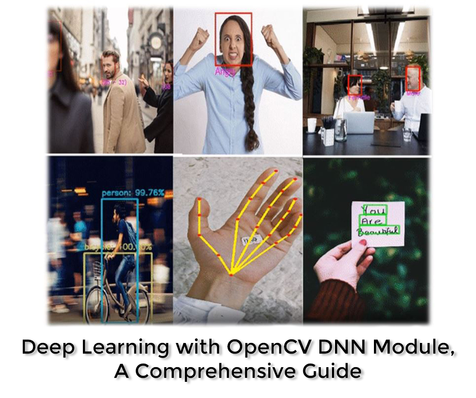
In this tutorial we will go over Deep learning using OpenCV’s DNN module in detail, I plan to cover various important details of the DNN module that is never discussed, things that usually trip of people like, selecting preprocessing params correctly and designing pre and postprocessing pipelines for different models.
This post is the first of 3 in our brand new Deep Learning with OpenCV series. All three posts are titled as:
Using a Caffe DenseNet121 model for classification.
Important Details regarding the DNN module, e.g. where to get models, how to configure them, etc.
If you’re just interested in the image classification part then you can skip to the second section or you can even read this great classification with DNN module post by Adrian. However, if you’re interested in getting to know the DNN module in all its glory then keep reading.
Introduction to OpenCV’s DNN module
First let me start by introducing the DNN module for all those people who are new to it, so as you can probably guess, the DNN module stands for Deep Neural Network module. This is the module in OpenCV which is responsible for all things deep learning related.
It was introduced in OpenCV version 3 and now in version 4.3, it has evolved a lot. This module lets you use pre-trained neural networks from popular frameworks like TensorFlow, PyTorch etc, and use those models directly in OpenCV.
This means you can train models using a popular framework like Tensorflow and then do inference/prediction with just OpenCV.
So what are the benefits here?
Here are some advantages you might want to consider when using OpenCV for inference.
By using OpenCV’s DNN module for inference the final code is a lot compact and simpler.
Someone who’s not familiar with the training framework can also use the model.
There are cases where using OpenCV’s DNN module will give you faster inference results for the CPU. See these results by Satya.
Beside supporting CUDA based NVIDIA’s GPU, OpenCV’s DNN module also supports OpenCL based Intel GPUs.
Most Importantly by getting rid of the training framework not only makes the code simpler but it ultimately gets rid of a whole framework, this means you don’t have to build your final application with a heavy framework like TensorFlow. This is a huge advantage when you’re trying to deploy on a resource-constrained edge device, e.g. a Raspberry pie.
One thing that might put you off is the fact that OpenCV can’t be used for training deep learning networks. This might sound like a bummer but fret not, for training neural networks you shouldn’t use OpenCV there are other specialized libraries like Tensorflow, PyTorch, etc for that task.
So which frameworks can you use to train Neural Networks:
These are the frameworks that are currently supported with the DNN module.
Now there are many interesting pre-trained models already available in the OpenCV Model Zoo that you can use, to keep things simple for this tutorial, I will be using an image classification network to do classification.
Details regarding other types of models are discussed in the 3rd section. By the way, I actually go over 13-14 different types of models in our Computer Vision and Image processing Course. These contain notebooks tutorials and video walk-throughs.
Image Classification pipeline with OpenCV DNN
Now we will be using a DenseNet121 model, which is a Caffe model trained on 1000 classes of ImageNet. The model is from the paper Densely Connected Convolutional Networks by Gap Huang et al.
Generally, there are 4 steps you need to perform when doing deep learning with the DNN module.
Read the image and the target classes.
Initialize the DNN module with an architecture and model parameters.
Perform the forward pass on the image with the module
Post-process the results.
The pre and post-processing steps are different for different tasks.
Let’s start with the code
Download Code
[optin-monster slug=”ag6ktwkaclnxqrmfitmo”]
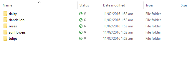
You can go ahead and download the source code from the download code section. After downloading the zip folder, unzip it and you will have the following directory structure.
Now run the Image Classification with DenseNet121.ipynb notebook, and start executing the cells.
Import Libraries
First, we will import the required libraries.
# Importing Required libraries
import numpy as np
import time
import cv2
import matplotlib.pyplot as plt
import os
import sys
Loading Class Labels
Now we’ll start by loading class names, In this notebook, we are going to classify among 1000 classes defined in ImageNet.
All these classes are in the text file named synset_words.txt. In this text file, each class is in on a new line with its unique id, Also each class has multiple labels for e.g look at the first 3 lines in the text file:
‘n01440764 tench, Tinca tinca’
‘n01443537 goldfish, Carassius auratus’
‘n01484850 great white shark, white shark
So for each line, we have the Class ID, then there are multiple class names, they all are valid names for that class and we’ll just use the first one. So in order to do that we’ll have to extract the second word from each line and create a new list, this will be our labels list.
# Split all the classes by a new line and store it in variable called rows.
rows = open('model/synset_words.txt').read().strip().split("n")

# Check the number of classes.
print("Number of Classes "+str(len(rows)))

# Show the first 5 rows
print(rows[0:5])
Number of Classes 1000
[‘n01440764 tench, Tinca tinca’, ‘n01443537 goldfish, Carassius auratus’, ‘n01484850 great white shark, white shark, man-eater, man-eating shark, Carcharodon carcharias’, ‘n01491361 tiger shark, Galeocerdo cuvieri’, ‘n01494475 hammerhead, hammerhead shark’]
Extract the Label
Here we will extract the labels (2nd element from each line) and create a labels list.
# Split by comma after first space is found and grabb the first element and store it in a new list.
CLASSES = [r[r.find(" ") + 1:].split(",")[0] for r in rows]

# Print the first 20 processed class labels
print(CLASSES[0:20])
prototxt: Path to the .prototxt file, this is the text description of the architecture of the model.
caffeModel: path to the .caffemodel file, this is your actual trained neural network model, it contains all the weights/parameters of the model. This is usually several MBs in size.
Note: If you load the model and proto file via readNetFromTensorFlow then the order of architecture and model inputs are reversed.
# Load the Model Weights.
weights = 'model/DenseNet_121.caffemodel'

# Load the Model Architecture.
architecture ='model/DenseNet_121.prototxt.txt'

# Here we are reading pre-trained caffe model with its architecture
net = cv2.dnn.readNetFromCaffe(architecture,weights)
Read An Image
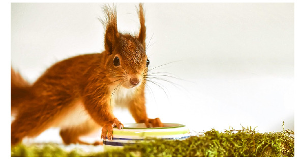
Let’s read an example image and display it with matplotlib imshow
# Load the input image
image = cv2.imread('images/jemma2.jpg')

# Display the image
plt.figure(figsize=(10,10))
plt.imshow(image[:,:,::-1]);plt.axis("off");
Pre-processing the image
Now before you pass an image in the network you need to preprocess it, this means resizing the image to the size it was trained on, for many networks, this is 224×224, in pre-processing step you also do other things like Normalize the image (make the range of intensity values between 0-1) and mean subtraction, etc. These are all the steps the authors did on the images that were used during model training.
Fortunately, In OpenCV, you have a function called cv2.dnn.blobFromImage() which most of the time takes care of all the pre-processing for you.
Scalefactor Used to normalize the image. This value is multiplied by the image, value of 1 means no scaling is done.
Size The size to which the image will be resized to, this depends upon the each model.
Mean These are mean R,G,B Channel values from the whole dataset and these are subtracted from the image’s R,G,B respectively, this gives illumination invariance to the model.
swapRB Boolean flag (false by default) this indicates weather swap first and last channels in 3-channel image is necessary.
crop flag which indicates whether the image will be cropped after resize or not. If crop is true, input image is resized so one side after resize is equal to the corresponding dimension in size and another one is equal or larger. Then, a crop from the center is performed. If crop is false, direct resize without cropping and preserving aspect ratio is performed.
So After this function, we get a 4d blob, this is what we’ll pass to the network.
print(blob.shape)
(1, 3, 224, 224)
Note: There is also blobFromImages() which does the same thing but with multiple images.
Input the Blob Image to the Network
Here you’re setting up the blob image as the input to the network.
# Passing the blob as input through the network
net.setInput(blob)
Forward Pass
Here the actual computation will take place, Most of the time in your whole pipeline will be taken here. Here your image will go through all the model parameters and in the end, you will get the output of the classifier.
%%time
Output = net.forward()
Wall time: 166 ms
# Length of the number of predictions
print("Total Number of Predictions are: {}".format(len(Output[0])))
By looking at the output, you can tell that the model has returned a set of scores for each class but we need Probabilities between 0-1 for each class. We can get them by applying a softmax function on the scores.
# Reshape the Output so its a single dimensional vector
new_Output = Output.reshape(len(Output[0][:]))

# Convert the scores to class probabilities between 0-1 by applying softmax
expanded = np.exp(new_Output - np.max(new_Output))
prob =  expanded / expanded.sum()
Now that we have understood step by step how to create the pipeline for classification using OpenCV’s DNN module, we’ll now create functions that do all the above in a single step. In short, we will be creating the following two functions.
Initialization Function: This function will contain parts of the network that will be set once, like loading the model.
Main Function: This function will contain all the rest of the code from preprocessing to postprocessing, it will also have the option to either return the image or display it with matplotlib.
Initialization Function
This method will be run once and it will initialize the network with the required files.
def init_classify(weights_name = 'DenseNet_121.caffemodel', architecture_name = 'DenseNet_121.prototxt.txt'):

    # Set global variables
    global net, classes

    base_path = 'model'

    # Read the Classes
    rows = open(os.path.join(base_path,'synset_words.txt')).read().strip().split("n")

    # Load and split  the classes
    classes = [r[r.find(" ") + 1:].split(",")[0] for r in rows]

    # Load the wieght and architeture of the model
    weights = os.path.join(base_path, weights_name)
    architecture = os.path.join(base_path, architecture_name)

    # Intialize the model
    net = cv2.dnn.readNetFromCaffe(architecture, weights)
Main Method
returndata is set to `True` when we want to perform classification on video.
def classify(image, returndata=False, size=1,):
# Pre-process the image
blob = cv2.dnn.blobFromImage(image, 0.017, (224, 224), (103.94,116.78,123.68))
# Input blob image into network
net.setInput(blob)
# Forward pass
Output = net.forward()
# Reshape the Output so its a single dimensional vector
new_Output = Output.reshape(len(Output[0][:]))
# Convert the scores to class probabilities between 0-1.
expanded = np.exp(new_Output - np.max(new_Output))
prob = expanded / expanded.sum()
# Get Highest probable class.
conf= np.max(prob)
# Index of Class with the maximum Probability.
index = np.argmax(prob)
# Name of the Class with the maximum probability
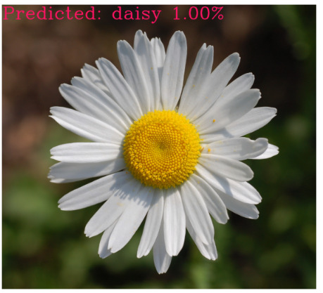
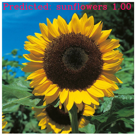
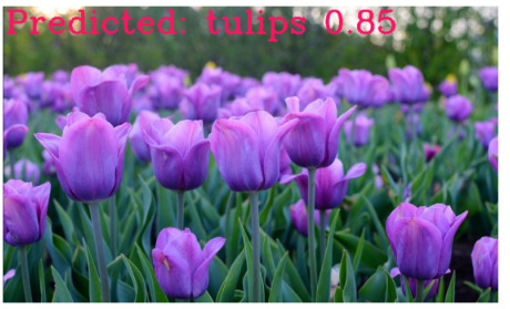
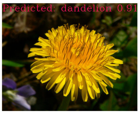
label = classes[index]
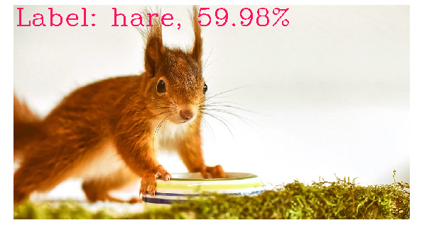
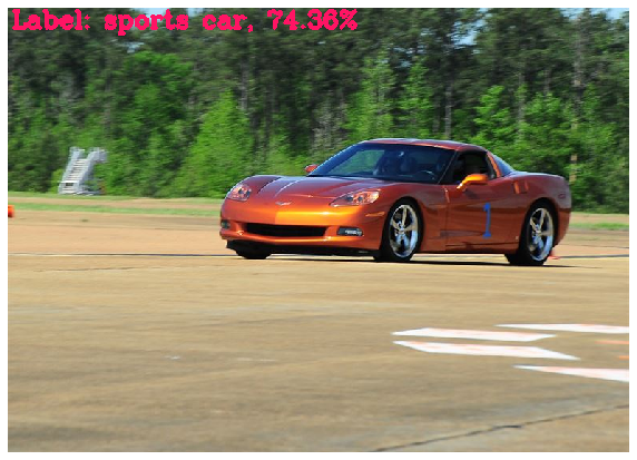
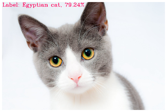
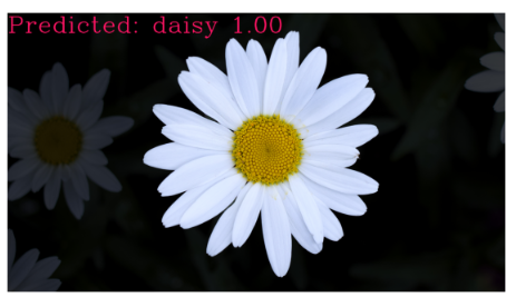
text = "Label: {}, {:.2f}%".format(label, conf*100)
cv2.putText(image, text, (5, size*26), cv2.FONT_HERSHEY_COMPLEX, size, (100, 20, 255), 3)
if returndata:
return image, text
else:
plt.figure(figsize=(10,10))
plt.imshow(image[:,:,::-1]);plt.axis("off");
Initialize the Classifier
Calling our initializer to initialize the network.
init_classify()
Using our Classifier Function
Now we can call our classifier function and test on multiple images.
If you want to this classifier in real-time then here is the code for that.
# Initialize fps to 0
fps = 0

# Load the classes and model
init_classify()

# Initialize the webcame
cap=cv2.VideoCapture(0)

while(True):

    # Fetch the inital time in order to find FPS
    start_time = time.time()

    # Read the frame from camera
    ret, frame=cap.read()

    # If camera is not working break the loop
    if not ret:
        break

    # Flip the frame, laterally
    image = cv2.flip(frame,1)

    # Classify the objects in frames
    image,_ = classify(image, returndata=True)

    # Display the classified object of frames
    cv2.putText(image, 'FPS: {:.2f}'.format(fps), (470, 20), cv2.FONT_HERSHEY_COMPLEX,0.8, (255, 20, 55), 2)

    # Display the window
    cv2.imshow("Image",image)

    # Calculate FPS
    fps = (1.0 / (time.time() - start_time))

    # Press `q` in order to close the window
    k = cv2.waitKey(1)
    if k == ord('q'):
        break

# Release the camera and destroy all opened windows
cap.release()
cv2.destroyAllWindows()
Important Details Regarding the DNN module
Let’s discuss some interesting details and some tips to fully utilize the DNN module.
Where to get the pre-trained Models:
Earlier I mentioned that you can get other pre-trained models, so where are they?
The best place to get pre-trained models is here. This page is a wiki for Deep learning with OpenCV, you will find models that have been tested by the OpenCV team.
There are a variety of models present here, for things like Classification, Pose Detection, Colorization, Segmentation, Face recognition, text detection, style transfer, and more. You can take models from any of the above 5 frameworks.
Just click on the models to go to their repo and download them from there. Note: The models listed on the page above are only the tested models, in theory, you can almost take any pre-trained model and use it in OpenCV.
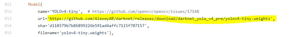
A faster and easier way to download models is to go here. Now, this is a python script that will let you download not only the most commonly used models but also some State of the Art ones like Yolo v4 etc. You can download this script and then run from the command line. Alternatively, if you’re in a rush and just one specific model then you can take the downloadable URL of any model and download it.
After downloading the model, you will need a couple of more things before you can actually use the model in the OpenCV dnn module.
You’re now probably familiar with those things, so yeah you will need the model configuration file like the prototxt file we just used with our Caffe model above. You will also need class labels, now for classification problems, models are usually trained on the ImageNet dataset so we needed synset_word.txt file, for Object detection you will find models trained on COCO or Pascal VOC dataset. And similarly, other tasks may require other files.
So where are all these files present?
You will find most of these configuration files present here and the class names here. If the configuration file you’re looking for is not present in the above links then I would recommend that you look at the GitHub repo of the model, the files would be present there. Otherwise, you have to create it yourself. (More on this later)
After getting the configuration files, the only thing you need is the pre-processing parameters that go in blobFromImage. E.g. the mean subtraction values, scaling params, etc.
You can get that information from here. Now, this script only contains parameter details for a few popular models.
So how do you get the details for other models?
For that you would need to go to the repo of the model and look in the ReadMe section, the authors usually put that information there.
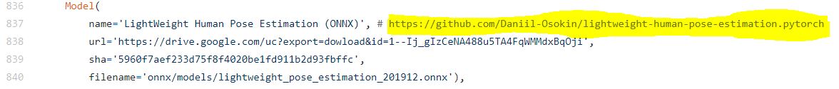
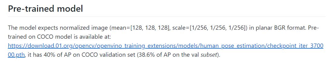
For e.g. If I visit the GitHub repo of the Human Pose Estimation model using this link which I got from the model downloading script.
By scrolling down the readme I can find these details here:
Note: These details are not always present in the Readme and sometimes you have to do quite some digging before you can find these parameters.
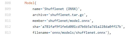
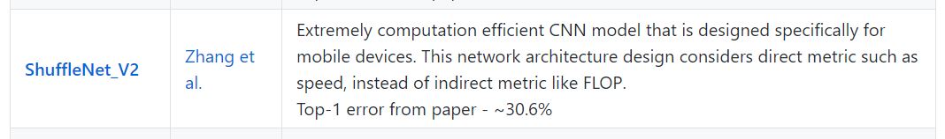
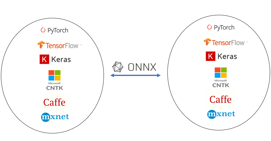
What to do if there is no GitHub repo link with the model, for e.g. this shuffleNet model does not have a GitHub link, in that case, I can see that the framework is ONNX.
So now I will visit the ONNX model zoo repo and find that model.
After clicking on the model I will find its readme and then its preprocessing steps.
Notice that this model contains some preprocessing steps that are not supported by blobfromImage function. So this could happen and at times you would need to write custom preprocessing steps without using blobfromImage function, for e.g. in our Super Resolution post, I had to write a custom pre-processing pipeline for the network.
How to use our own Custom Trained Networks
Now that we have learned to use different models, you might wonder exactly how can we use our own custom-trained models. So the thing is you can’t directly plug a trained network in a DNN module but you need to perform some operations to get a configuration file, which is why we needed a prototxt file along with the model.
Fortunately, In the next two blog posts, I plan to cover exactly this topic and show you how to use a custom trained classifier and a custom trained Detection network.
For now, you can take a look at this page which briefly describes how you can use models trained with Tensorflow Object Detection API in OpenCV.
One thing to note is that not all networks are supported by the DNN module, this is because the DNN module supports some 30+ layer types, these layer names can be found at the wiki here. So if a model contains layers that are not among the supported layers then it won’t run, this is not a major issue as most common layers used in deep learning models are supported.
Using GPU’s and Faster Backends to speed up OpenCV DNN Module
By default OpenCV’s DNN deep learning module runs on the default C++ implementation which itself is pretty fast but OpenCV further allows you to change this backend to increase the speed even more.
Option 1: Use NVIDIA GPU with CUDA backend in the DNN module:
If you have an Nvidia GPU present then great, you can use that with the DNN module, you can follow my OpenCV source installation guide to configure your NVIDIA GPU for OpenCV and learn how to use it. This will make your networks run several times faster.
Option 2: Use OpenCL based INTEL GPU’s:
If you have an OpenCL-based GPU then you can use that as a backend, although this increases speed but in my experience, I’ve seen speed gains only in 32 bit systems. To use the OpenCL as a backend you can see the last section of my OpenCV source installation section linked above.
Option 3: Use Halide Backend:
As described in this post from learnOpenCV.com, for some time in the past using the halide backend increased the speed but then OpenCV engineer’s optimized the default C++ implementation so much that the default implementation actually got faster. So I don’t see a reason to use this backend now, Still here’s how you configure halide as a backend.
Option 4: Use Intel’s Deep Learning Inference Engine backend:
Intel’s Deep Learning Inference Engine backend is part of the OpenVINO toolkit, OpenVINO stands for Open Visual Inferencing and Neural Network Optimization. OpenVINO is designed by Intel to speed up inference with neural networks, especially for tasks like classification, detection, etc. OpenVINO speeds up by optimizing the model in a hardware-agnostic way. You can learn to install OpenVINO here and here’s a nice tutorial for it.
Hire Us
Let our team of expert engineers and managers build your next big project using Bleeding Edge AI Tools & Technologies
In today’s tutorial, we went over a number of things regarding OpenCV’s DNN module. From using pre-trained models to Optimizing for faster inference speed.
We also learned to perform a classification pipeline using densenet121.
This post should serve as an excellent guide for anyone trying to get started in Deep learning using OpenCV’s DNN module.
Finally, OpenCV’s DNN repo contains an example python script to run common networks like classification, text, object detection, and more. You can start utilizing the DNN module by using these scripts and here are a few DNN Tutorials by OpenCV.
The main contributor for the DNN module in OpenCV is Dmitry Kurtaev and formerly it was Aleksandr Rybnikov, so big thanks to them and the rest of the contributors for making such a great module.
I hope you enjoyed today’s tutorial, feel free to comment and ask questions.
You can reach out to me personally for a 1 on 1 consultation session in AI/computer vision regarding your project. Our talented team of vision engineers will help you every step of the way. Get on a call with me directlyhere.
Ready to seriously dive into State of the Art AI & Computer Vision? Then Sign up for these premium Courses by Bleed AI
You can reach out to me personally for a 1 on 1 consultation session in AI/computer vision regarding your project. Our talented team of vision engineers will help you every step of the way. Get on a call with me directlyhere.
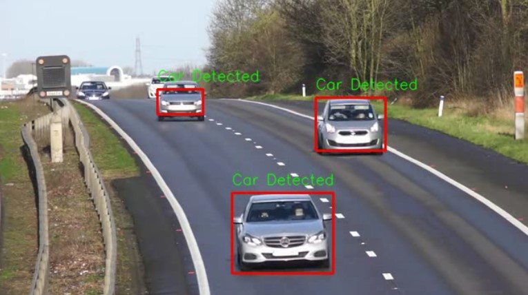
Let’s say you have been tasked to design a system capable of detecting vehicles on a road such as the one below,
Surely, this seems like a job for a Deep Neural Network, right?
This means you have to get a lot of data, label them, then train a model, tune its performance and serve it on a system capable of running it in real-time.
This sounds like a lot of work and it begs the question: Is deep learning the only way to do so?
What if I tell you that you can solve this problem and many others like this using a much simpler approach, and with this approach, you will not have to spend days collecting data or training deep learning models. And the approach is also lightweight so it will run on almost any machine!
Alright, what exactly are we talking about here?
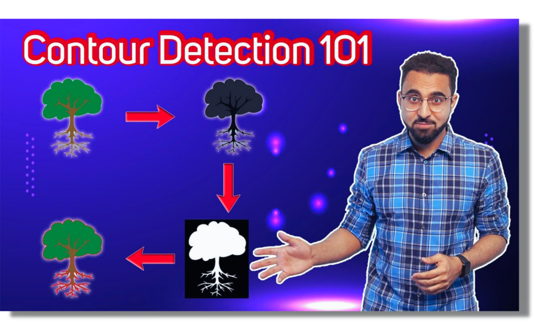
This simpler approach relies on a popular Computer Vision technique called Contour Detection. A handy technique that can save the day when dealing with vision problems such as the one above. Although not as generalizable as Deep Neural Networks, contour detection can prove robust under controlled circumstances, requiring minimum time investment and effort to build vision applications.
Just to give you a glimpse of what you can build with contour detection, have a look at some of the applications that I made using contour detection.
and there are many other applications that you can build too, once you learn about what contour Detection is and how you can use it, in fact, I have an entire course that will help you master contours for building computer vision applications.
Since Contours is a lengthy topic, I’ll be breaking down Contours into a 4 parts series. This is the first part where we discuss the basics of contour detection in OpenCV, how to use it, and go over various preprocessing techniques required for Contour Detection.
A contour can be simply defined as a curve that joins a set of points enclosing an area having the same color or intensity. This area of uniform color or intensity forms the object that we are trying to detect, and the curve enclosing this area is the contour representing the shape of the object. So essentially, contour detection works similarly to edge-detection but with the restriction that the edges detected must form a closed path.
Still confused? Just have a look at the GIF below. You can see four shapes, which on a pixel level forms when certain pixels share the same color which is distinct from the background color. Contour detection identifies each of the border pixels that is distinct from the background forming an enclosed, continuous path of pixels that form the line representing the contour.
Now, let’s see how this works in OpenCV.
Import the Libraries
Let’s start by importing the required libraries.
import cv2
import numpy as np
import matplotlib.pyplot as plt
Read an Image
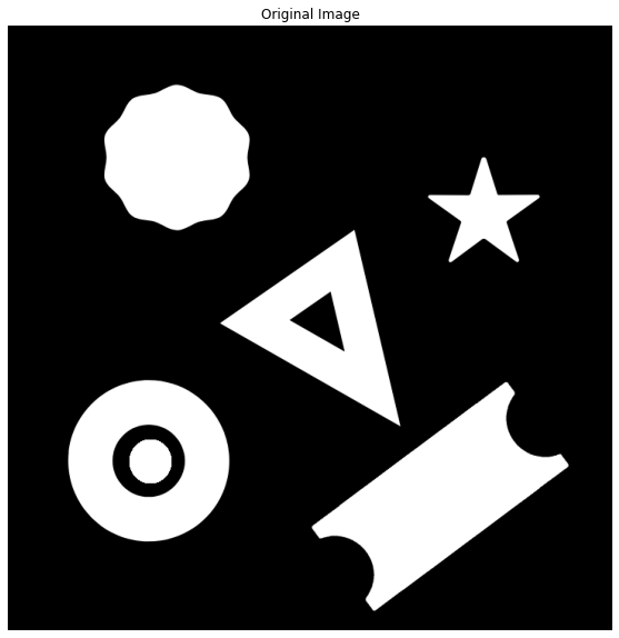
Next, we will read an image below containing a bunch of shapes for which we will find the contours.
# Read the image
Gray_image = cv2.imread('media/image.png', 0)

# Display the image
plt.figure(figsize=[10,10])
plt.imshow(image1, cmap='gray');plt.title("Original Image");plt.axis("off");
OpenCV saves us the trouble of writing lengthy algorithms for contour detection and provides a handy function findContours() that analyzes the topological structure of the binary image by border following, a contour detection technique developed in 1985.
The findContours() function takes a binary image as input. The foreground is assumed to be white, and the background is assumed to be black. If that is not the case, then you can invert the image pixels using the cv2.bitwise_not() function.
image – It is the input image (8-bit single-channel). Non-zero pixels are treated as 1’s. Zero pixels remain 0’s, so the image is treated as binary. You can use compare, inRange, threshold, adaptiveThreshold, Canny, and others to create a binary image out of a grayscale or color one.
mode – It is the contour retrieval mode, ( RETR_EXTERNAL, RETR_LIST, RETR_CCOMP, RETR_TREE )
method – It is the contour approximation method. ( CHAIN_APPROX_NONE, CHAIN_APPROX_SIMPLE, CHAIN_APPROX_TC89_L1, etc )
offset – It is the optional offset by which every contour point is shifted. This is useful if the contours are extracted from the image ROI, and then they should be analyzed in the whole image context.
Returns:
contours – It is the detected contours. Each contour is stored as a vector of points.
hierarchy – It is the optional output vector containing information about the image topology. It has been described in detail in the video above.
We will go through all the important parameters in a while. For now, let’s detect some contours in the image that we read above.
Since the image read above only contains a single channel instead of three, and even that channel is in the binary state (black & white) so it can be directly passed to the findContours() function without requiring any preprocessing.
# Find all contours in the image.
contours, hierarchy = cv2.findContours(Gray_image, cv2.RETR_EXTERNAL, cv2.CHAIN_APPROX_SIMPLE)

# Display the total number of contours found.
print("Number of contours found = {}".format(len(contours)))
Number of contours found = 5
Visualizing the Contours detected
As you can see the cv2.findContours() function was able to correctly detect the 5 external shapes in the image. But how do we know that the detections were correct? Thankfully we can easily visualize the detected contours using the cv2.drawContours() function which simply draws the detected contours onto an image.
image – It is the image on which contours are to be drawn.
contours – It is point vector(s) representing the contour(s). It is usually an array of contours.
contourIdx – It is the parameter, indicating a contour to draw. If it is negative, all the contours are drawn.
color – It is the color of the contours.
thickness – It is the thickness of lines the contours are drawn with. If it is negative (for example, thickness=FILLED ), the contour interiors are drawn.
lineType – It is the type of line. You can find the possible options here.
hierarchy – It is the optional information about hierarchy. It is only needed if you want to draw only some of the contours (see maxLevel ).
maxLevel – It is the maximal level for drawn contours. If it is 0, only the specified contour is drawn. If it is 1, the function draws the contour(s) and all the nested contours. If it is 2, the function draws the contours, all the nested contours, all the nested-to-nested contours, and so on. This parameter is only taken into account when there is a hierarchy available.
offset – It is the optional contour shift parameter. Shift all the drawn contours by the specified offset=(dx, dy).
Let’s see how it works.
# Read the image in color mode for drawing purposes.
image1 = cv2.imread('media/image.png')

# Make a copy of the source image.
image1_copy = image1.copy()

# Draw all the contours.
cv2.drawContours(image1_copy, contours, -1, (0,255,0), 3)

# Display the result
plt.figure(figsize=[10,10])
plt.imshow(image1_copy[:,:,::-1]);plt.axis("off");
This seems to have worked nicely. But again, this is a pre-processed image that is easy to work with, which will not be the case when working with a real-world problem where you will have to pre-process the image before detecting contours. So let’s have a look at some common pre-processing techniques below.
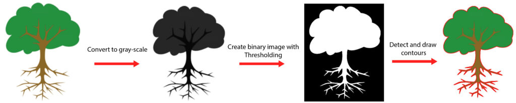
Pre-processing images For Contour Detection
As you have seen above that the cv2.findContours() functions takes in as input a single channel binary image, however, in most cases the original image will not be a binary image. Detecting contours in colored images require pre-processing to produce a single-channel binary image that can be then used for contour detection. Ideally, this processed image should have the target objects in the foreground.
The two most commonly used techniques for this pre-processing are:
Thresholding based Pre-processing
Edge Based Pre-processing
Below we will see how you can accurately detect contours using these techniques.
Thresholding based Pre-processing For Contours
So to detect contours in colored images we can perform fixed level image thresholding to produce a binary image, that can be then used for contour detection. Let’s see how this works.
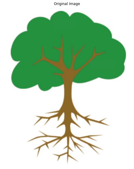
First, read a sample image using the function cv2.imread() and display the image using the matplotlib library.
# Read the image
image2 = cv2.imread('media/tree.jpg')

# Display the image
plt.figure(figsize=[10,10])
plt.imshow(image2[:,:,::-1]);plt.title("Original Image");plt.axis("off");
We will try to find the contour for the tree above, first without using any thresholding to see how the result will look like.
The first step is to convert the 3-channel BGR image to a single-channel image using the cv2.cvtColor() function.
# Make a copy of the source image.
image2_copy = image2.copy()

# Convert the image to gray-scale
gray = cv2.cvtColor(image2_copy, cv2.COLOR_BGR2GRAY)

# Display the result
plt.imshow(gray, cmap="gray");plt.title("Gray-scale Image");plt.axis("off");
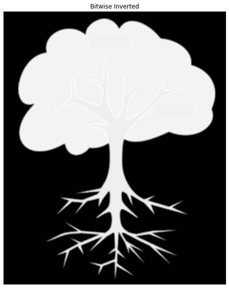
Contour detection on the image above will only result in a contour outlining the edges of the image. This is because the cv2.findContours() function expects the foreground to be white, and the background to be black, which is not the case above so we need to invert the colors using cv2.bitwise_not().
# Invert the colours
gray_inverted = cv2.bitwise_not(gray)

# Display the result
plt.figure(figsize=[10,10])
plt.imshow(gray_inverted ,cmap="gray");plt.title("Bitwise Inverted");plt.axis("off");
The inverted image with a black background and white foreground can now be used for contour detection.
# Find the contours from the inverted gray-scale image
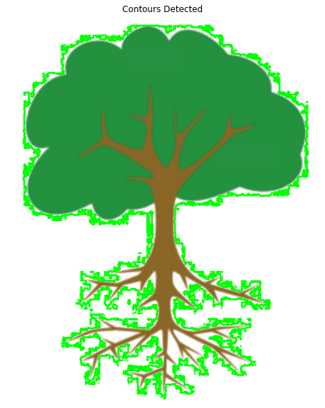
contours, hierarchy = cv2.findContours(gray_inverted, cv2.RETR_EXTERNAL, cv2.CHAIN_APPROX_NONE)
# draw all contours
cv2.drawContours(image2_copy, contours, -1, (0, 255, 0), 2)
# Display the result
plt.figure(figsize=[10,10])
plt.imshow(image2_copy[:,:,::-1]);plt.title("Contours Detected");plt.axis("off");
The result is far from ideal. As you can see the contours detected poorly align with the boundary of the tree in the image. This is because we only fulfilled the requirement of a single-channel image, but we did not make sure that the image was binary in colors, leaving noise along the edges. This is why we need thresholding to provide us a binary image.
Thresholding the image
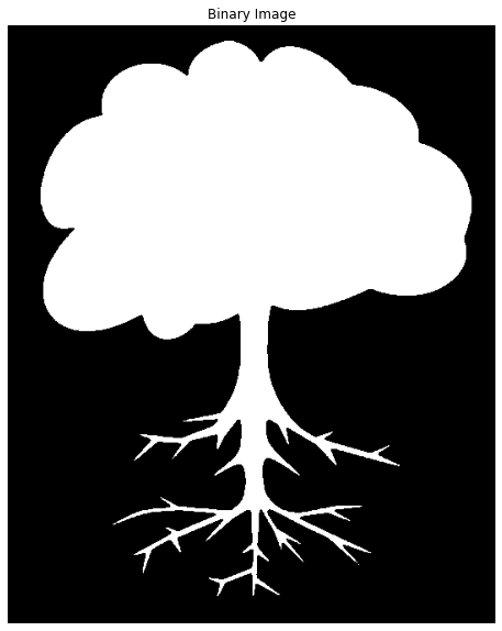
We will use the function cv2.threshold() to perform thresholding. The function takes in as input the gray-scale image, applies fixed level thresholding, and returns a binary image. In this case, all the pixel values below 100 are set to 0(black) while the ones above are set to 255(white). Since the image has already been inverted, cv2.THRESH_BINARY is used, but if the image is not inverted, cv2.THRESH_BINARY_INV should be used. Also, the fixed level used must be able to correctly segment the target object as foreground(white).
# Create a binary thresholded image
_, binary = cv2.threshold(gray_inverted, 100, 255, cv2.THRESH_BINARY)

# Display the result
plt.figure(figsize=[10,10])
plt.imshow(binary, cmap="gray");plt.title("Binary Image");plt.axis("off");
The resultant image above is ideally what the cv2.findContours() function is expecting. A single-channelbinary image with Black background and white foreground.
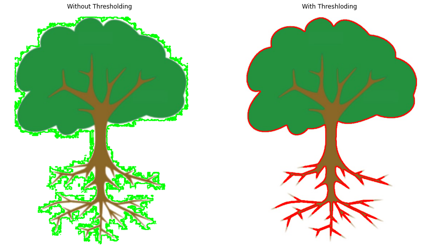
# Make a copy of the source image.
image2_copy2 = image2.copy()

# find the contours from the thresholded image
contours, hierarchy = cv2.findContours(binary, cv2.RETR_LIST, cv2.CHAIN_APPROX_SIMPLE)

# draw all the contours found
image2_copy2 = cv2.drawContours(image2_copy2, contours, -1, (0, 0, 255), 2)

# Plot both of the resuts for comparison
plt.figure(figsize=[15,15])
plt.subplot(121);plt.imshow(image2_copy[:,:,::-1]);plt.title("Without Thresholding");plt.axis('off')
plt.subplot(122);plt.imshow(image2_copy2[:,:,::-1]);plt.title("With Threshloding");plt.axis('off');
The difference is clear. Binarizing the image helps get rid of all the noise at the edges of objects, resulting in accurate contour detection.
Edge Based Pre-processing For Contours
Thresholding works well for simple images with fewer variations in colors, however, for complex images, it’s not always easy to do background-foreground segmentation using thresholding. In these cases creating the binary image using edge detection yields better results.
Let’s read another sample image.
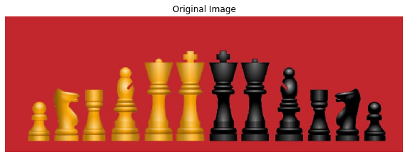
# Read the image
image3 = cv2.imread('media/chess.jpg')

# Display the image
plt.figure(figsize=[10,10])
plt.imshow(image3[:,:,::-1]);plt.title("Original Image");plt.axis("off");
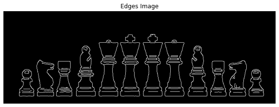
It’s obvious that simple fixed level thresholding wouldn’t work for this image. You will always end up with only half the chess pieces in the foreground only. So instead we will use the function cv2.Canny() for detecting the edges in the image. cv2.Canny() returns a single channel binary image which is all we need to perform contour detection in the next step. We also make use of the cv2.GaussianBlur() function to smoothen any noise in the image.
# Blur the image to remove noise
blurred_image = cv2.GaussianBlur(image3.copy(),(5,5),0)

# Apply canny edge detection
edges = cv2.Canny(blurred_image, 100, 160)

# Display the resultant binary image of edges
plt.figure(figsize=[10,10])
plt.imshow(edges,cmap='Greys_r');plt.title("Edges Image");plt.axis("off");
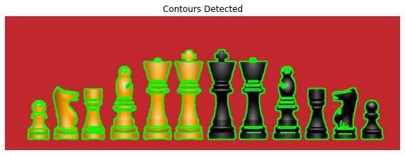
Now, using the edges detected, we can perform contour detection.
# Detect the contour using the edges
contours, hierarchy = cv2.findContours(edges, cv2.RETR_EXTERNAL, cv2.CHAIN_APPROX_SIMPLE)

# Draw the contours
image3_copy = image3.copy()
cv2.drawContours(image3_copy, contours, -1, (0, 255, 0), 2)

# Display the drawn contours
plt.figure(figsize=[10,10])
plt.imshow(image3_copy[:,:,::-1]);plt.title("Contours Detected");plt.axis("off");
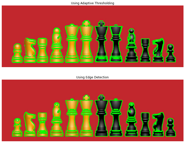
In comparison, if we were to use thresholding as before it would yield a poor result that will only manage to correctly outline half of the chess pieces in the image at a time. So for a fair comparison, we will use cv2.adaptiveThreshold() to perform adaptive thresholding which adjusts to different color intensities in the image.
image3_copy2 = image3.copy()

# Remove noise from the image
blurred = cv2.GaussianBlur(image3_copy2,(3,3),0)

# Convert the image to gray-scale
gray = cv2.cvtColor(blurred, cv2.COLOR_BGR2GRAY)

# Perform adaptive thresholding
binary = cv2.adaptiveThreshold(gray,255,cv2.ADAPTIVE_THRESH_GAUSSIAN_C,cv2.THRESH_BINARY_INV, 11, 5)

# Detect and Draw contours
contours, hierarchy = cv2.findContours(binary, cv2.RETR_EXTERNAL, cv2.CHAIN_APPROX_SIMPLE)
cv2.drawContours(image3_copy2, contours, -1, (0, 255, 0), 2)

# Plotting both results for comparison
plt.figure(figsize=[14,10])
plt.subplot(211);plt.imshow(image3_copy2[:,:,::-1]);plt.title("Using Adaptive Thresholding");plt.axis('off')
plt.subplot(212);plt.imshow(image3_copy[:,:,::-1]);plt.title("Using Edge Detection");plt.axis('off');
As can be seen above, using canny edge detection results in finer contour detection.
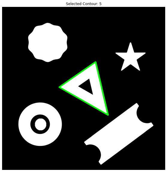
Drawing a selected Contour
So far we have only drawn all of the detected contours in an image, but what if we want to only draw certain contours?
The contours returned by the cv2.findContours() is a python list where the ith element is the contour for a certain shape in the image. Therefore if we are interested in just drawing one of the contours we can simply index it from the contours list and draw the selected contour only.
image1_copy = image1.copy()

# Find all contours in the image.
contours, hierarchy = cv2.findContours(Gray_image, cv2.RETR_LIST, cv2.CHAIN_APPROX_NONE)

# Select a contour
index = 5
contour_selected = contours[index]

# Draw the selected contour
cv2.drawContours(image1_copy, contour_selected, -1, (0,255,0), 6);

# Display the result
plt.figure(figsize=[10,10])
plt.imshow(image1_copy[:,:,::-1]);plt.axis("off");plt.title('Selected Contour: ' + str(index));
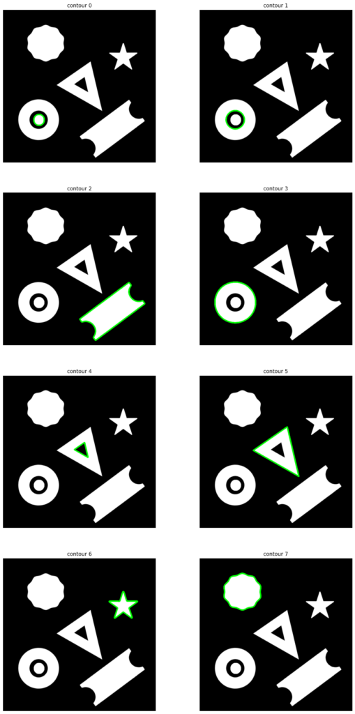
Now let’s modify our code using a for loop to draw all of the contours separately.
image1_copy = image1.copy()

# Create a figure object for displaying the images
plt.figure(figsize=[15,30])

# Convert to grayscale.
imageGray = cv2.cvtColor(image1_copy,cv2.COLOR_BGR2GRAY)

# Find all contours in the image
contours, hierarchy = cv2.findContours(imageGray, cv2.RETR_LIST, cv2.CHAIN_APPROX_NONE)

# Loop over the contours
for i,cont in enumerate(contours):

        # Draw the ith contour
        image1_copy = cv2.drawContours(image1.copy(), cont, -1, (0,255,0), 6)

        # Add a subplot to the figure
        plt.subplot(4, 2, i+1)

        # Turn off the axis
        plt.axis("off");plt.title('contour ' +str(i))

        # Display the image in the subplot
        plt.imshow(image1_copy)
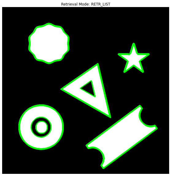
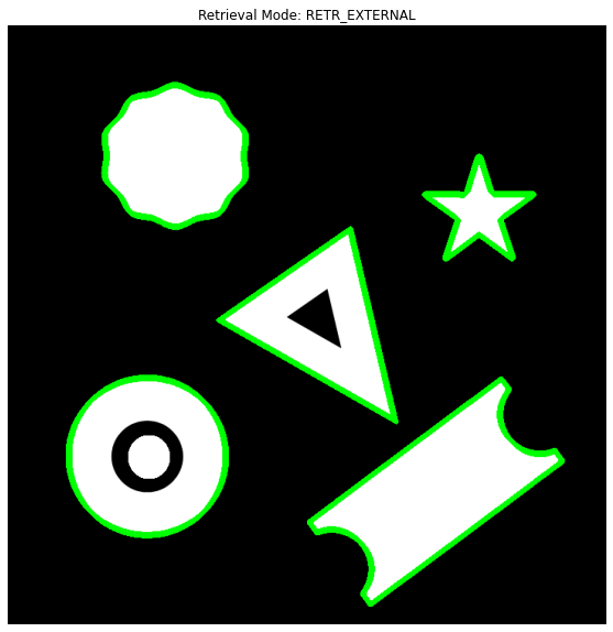
Retrieval Modes
Function cv2.findContours() does not only returns the contours found in an image but also returns valuable information about the hierarchy of the contours in the image. This hierarchy encodes how the contours may be arranged in the image, e.g, they may be nested within another contour. Often we are more interested in some contours than others. For example, you may only want to retrieve the external contour of an object.
Using the Retrieval Modes specified, the cv2.findContours() function can determine how the contours are to be returned or arranged in a hierarchy.
For more information on Retrieval modes and contour hierarchy Read here.
Some of the important retrieval modes are:
cv2.RETR_EXTERNAL – retrieves only the extreme outer contours.
cv2.RETR_LIST – retrieves all of the contours without establishing any hierarchical relationships.
cv2.RETR_TREE – retrieves all of the contours and reconstructs a full hierarchy of nested contours.
cv2.RETR_CCOMP – retrieves all of the contours and organizes them into a two-level hierarchy. At the top level, there are external boundaries of the components. At the second level, there are boundaries of the holes. If there is another contour inside a hole of a connected component, it is still put at the top level.
Below we will have a look at how each of these modes return the contours.
cv2.RETR_LIST
cv2.RETR_LIST simply retrieves all of the contours without establishing any hierarchical relationships between them. All of the contours can be said to have no parent or child relationship with another contour.
image1_copy = image1.copy()

# Convert to gray-scale
imageGray = cv2.cvtColor(image1_copy, cv2.COLOR_BGR2GRAY)

# Find and return all contours in the image using the RETR_LIST mode
contours, hierarchy = cv2.findContours(imageGray, cv2.RETR_LIST, cv2.CHAIN_APPROX_SIMPLE)

# Draw all contours.
cv2.drawContours(image1_copy, contours, -1, (0,255,0), 3);

# Print the number of Contours returned
print("Number of Contours Returned: {}".format(len(contours)))

# Display the results.
plt.figure(figsize=[10,10])
plt.imshow(image1_copy);plt.axis("off");plt.title('Retrieval Mode: RETR_LIST');
Number of Contours Returned: 8
cv2.RETR_EXTERNAL
cv2.RETR_EXTERNAL retrieves only the extreme outer contours i.e the contours not having any parent contour.
image1_copy = image1.copy()

# Find all contours in the image.
contours, hierarchy = cv2.findContours(imageGray, cv2.RETR_EXTERNAL, cv2.CHAIN_APPROX_SIMPLE)

# Draw all the contours.
cv2.drawContours(image1_copy, contours, -1, (0,255,0), 3);

# Print the number of Contours returned
print("Number of Contours Returned: {}".format(len(contours)))

# Display the results.
plt.figure(figsize=[10,10])
plt.imshow(image1_copy);plt.axis("off");plt.title('Retrieval Mode: RETR_EXTERNAL');
Number of Contours Returned: 5
cv2.RETR_TREE
cv2.RETR_TREE retrieves all of the contours and constructs a full hierarchy of nested contours.
src_copy = image1.copy()

# Convert to gray-scale
imageGray = cv2.cvtColor(src_copy,cv2.COLOR_BGR2GRAY)

# Find all contours in the image while maintaining a hierarchy
contours, hierarchy = cv2.findContours(imageGray, cv2.RETR_TREE, cv2.CHAIN_APPROX_SIMPLE)

# Draw all the contours.
contour_image = cv2.drawContours(src_copy, contours, -1, (0,255,0), 3);

# Print the number of Contours returned
print("Number of Contours Returned: {}".format(len(contours)))

# Display the results.
plt.figure(figsize=[10,10])
plt.imshow(contour_image);plt.axis("off");plt.title('Retrieval Mode: RETR_TREE');
Number of Contours Returned: 8
cv2.RETR_CCOMP
cv2.RETR_CCOMP retrieves all of the contours and organizes them into a two-level hierarchy. At the top level, there are external boundaries of the object. At the second level, there are boundaries of the holes in object. If there is another contour inside that hole, it is still put at the top level.
To visualize the two levels we check for the contours that do not have any parent i.e the fourth value in their hierarchy [Next, Previous, First_Child, Parent] is set to -1. These contours form the first level and are represented with green color while all other are second-level contours represented in red.
src_copy = image1.copy()
imageGray = cv2.cvtColor(src_copy,cv2.COLOR_BGR2GRAY)

# Find all contours in the image using RETE_CCOMP method
contours, hierarchy = cv2.findContours(imageGray, cv2.RETR_CCOMP, cv2.CHAIN_APPROX_NONE)

# Loop over all the contours detected
for i,cont in enumerate(contours):

    # If the contour is at first level draw it in green
    if hierarchy[0][i][3] == -1:
        src_copy = cv2.drawContours(src_copy, cont, -1, (0,255,0), 3)

    # else draw the contour in Red
    else:
        src_copy = cv2.drawContours(src_copy, cont, -1, (255,0,0), 3)

# Print the number of Contours returned
print("Number of Contours Returned: {}".format(len(contours)))

# Display the results.
plt.figure(figsize=[10,10])
plt.imshow(src_copy);plt.axis("off");plt.title('Retrieval Mode: RETR_CCOMP');
Number of Contours Returned: 8
[optin-monster slug=”d8wgq6fdm5mppdb5fi99″]
Summary
Alright, In the first part of the series we have unpacked a lot of important things about contour detection and how it works. We discussed what types of applications you can build using Contour Detection and the circumstances under which it works most effectively.
We saw how you can effectively detect contours and visualize them too using OpenCV.
The post also went over some of the most common pre-processing techniques used prior to contour detection.
Thresholding based Pre-processing
Edge Based Pre-processing
which will help you get accurate results with contour detection. But these are not the only contour detection techniques, ultimately, it depends on what type of problem you are trying to solve, and figuring out the appropriate pre-processing to use is the key to contour detection. Start by asking what properties distinguish the target object from the rest of the image? Then figure out the best way you can use to isolate those properties.
We also went over the important Retrieval Modes that can be used to change how the hierarchy of the detected contours works or even change what type of contours are detected. Additionally, you can always use the hierarchy to only extract the contours you want, e.g. retrieve only the contours at level three.
This was the first part of the series but there are four more to come in which we will dive deeper into contour detection with OpenCV and also build a cool vision application using contour Detection!
You can reach out to me personally for a 1 on 1 consultation session in AI/computer vision regarding your project. Our talented team of vision engineers will help you every step of the way. Get on a call with me directlyhere.
Ready to seriously dive into State of the Art AI & Computer Vision? Then Sign up for these premium Courses by Bleed AI
In the previous tutorial we learned how the DNN module in OpenCV works, we went into a lot of details regarding different aspects of the module including where to get the models, how to configure them, etc.
This Tutorial will build on top of the previous one so if you haven’t read the previous post then you can read that here.
Today’s post is the second tutorial in our brand new 3 part Deep Learning with OpenCV series. All three posts are titled as:
In this post, we will train a custom image classifier with Tensorflow’s Keras API. So if you want to learn how to get started creating a Convolutional Neural Network using Tensorflow, then this post is for you, and not only that but afterward, we will also convert our trained .h5 model to ONNX format and then use it with OpenCV DNN module.
Converting your model to onnx will give you more than a 3x reduction in model size.
This whole process shows you how to train models in Tensorflow and then deploy them directly in OpenCV.
What’s the advantage of using the trained model in OpenCV vs using it in Tensorflow?
So here are some points you may want to consider.
By using OpenCV’s DNN module, the final code is a lot compact and simpler.
Someone who’s not familiar with the training framework like TensorFlow can also use this model.
Besides supporting CUDA based NVIDIA’s GPU, OpenCV’s DNN module also supports OpenCL based Intel GPUs.
Most Importantly by getting rid of the training framework (Tensorflow) not only makes the code simpler but it ultimately gets rid of a whole framework, this means you don’t have to build your final application with a heavy framework like TensorFlow. This is a huge advantage when you’re trying to deploy on a resource-constrained edge device, e.g. a Raspberry pie
So this way you’re getting the best of both worlds, a framework like Tensorflow for training and OpenCV DNN for faster inference during deployment.
This tutorial can be split into 3 parts.
Training a Custom Image Classifier in OpenCV with Tensorflow
Converting Our Classifier to ONNX format.
Using the ONNX model directly in the OpenCV DNN module.
Let’s start with the Code
Download Code
[optin-monster slug=”scb99lhehb40udr0ckhj”]
Part 1: Training a Custom Image Classifier with Tensorflow:
For this tutorial you need OpenCV4.0.0.21 and Tensorflow 2.2
So you should do:
pip install opencv-contrib-python==4.0.0.21 (Or install from Source, Make sure to change the version)
Note: The reason I’m asking you to install version 4.0 instead of the latest 4.3 version of OpenCV is that later on, we’ll be using a function called readNetFromONNX() now with our model this function was giving an error in 4.3 and 4.2, possibly due to some bug in those versions. This does not mean that you can’t use custom models with those versions but that for my specific case there was an issue. Converting models only takes 2-3 lines of code but sometimes you get ambiguous errors that are hard to diagnose, but it can be done.
Hopefully, the conversion process will get better in the future.
One thing you can do is create a custom environment (with Anaconda or virtualenv) in which you can install version 4.0 without affecting your root environment and if you’re using google colab for this tutorial then you don’t need to worry about that.
You can go ahead and download the source code from the download code section. After downloading the zip folder, unzip it and you will have the following directory structure.
# Import Required libraries
import tensorflow as tf
from tensorflow.keras.models import Sequential, load_model, Model
from tensorflow.keras.layers import Dense, Conv2D, Dropout, MaxPooling2D, GlobalAveragePooling2D, Activation
from tensorflow.keras.preprocessing.image import ImageDataGenerator
from tensorflow.keras.optimizers import Adam
import os
import numpy as np
import cv2
import matplotlib.pyplot as plt
import urllib.request
import tarfile
Let’s see how you would go about training a basic Convolutional Network in Tensorflow. I assume you know some basics of deep learning. Also in this tutorial, I will be teaching how to construct and train a classifier using a real-world dataset, not a toy one, I will not go in-depth and explain the theory behind neural networks. If you want to start learning deep learning then you can take a look at Andrew Ng’s Deep Learning specialization, although this specialization is basic and covers mostly foundational things now if your end goal is to specialize in computer Vision then I would strongly recommend that you first learn Image Processing and Classical Computer Vision techniques from my 3-month comprehensive course here.
The Dataset we’re going to use here is a dataset of 5 different flowers, namely rose, tulips, sunflower, daisy, and dandelion. I avoided the usual cats and dogs dataset.
You can download the dataset from a URL, you just have to run this cell
After extracting you can check the folder named flower_photos in your current directory which will contain these 5 subfolders.
You can check the number of images in each class using the code below.
# This is the directory path where all the class folders are
dir_path =  'flower_photos'

# Initialize classes list, this list will contain the names of our classes.
classes = []

# Iterate over the names of each class
for class_name in os.listdir(dir_path):

   # Get the full path of each class
  class_path = os.path.join(dir_path, class_name)

  # Check if the class is a directory/folder
  if os.path.isdir(class_path):

      # Get the number of images in each class and print them
      No_of_images = len(os.listdir(class_path))
      print("Found {} images of {}".format(No_of_images , class_name))

      # Also store the name of each class
      classes.append(class_name)

# Sort the list in alphabatical order and print it
classes.sort()
print(classes)
Found 699 images of sunflowers Found 898 images of dandelion Found 633 images of daisy Found 799 images of tulips Found 641 images of roses [‘daisy’, ‘dandelion’, ‘roses’, ‘sunflowers’, ‘tulips’]
Generate Images:
Now it’s time to load up the data, now since the data is approx 218 MB, we can actually load it in RAM but most real datasets are large several GBs in size, and will fit in your RAM. In those scenarios, you use data generators to fetch batches of data and feed it to the neural network during training, so today we’ll also be using a data generator to load the data.
Before we can pass the images to a deep learning model, we need to do some preprocessing, like resizing the image in the required shape, converting them to floating-point tensors, rescale the pixel values from 0-255 to 0-1 range as this helps in training.
Fortunately, all of this can be done by the ImageDataGenerator class in tf.keras. Not only that but the ImageDataGenerator Class can also perform data augmentation. Data augmentation means that the generator takes your image and performs random transformations like randomly rotating, zooming, translating, and performing other such operations to the image. This is really effective when you don’t have much data as this increases your dataset size on the fly and your dataset contains more variation which helps in generalization.
As you’ve already seen that each flower class has less than 1000 examples, so in our case data augmentation will help a lot. It will expand our dataset.
When training a Neural Network, we normally use 2 datasets, a training dataset, and a validation dataset. The neural network tunes its parameters using the training dataset and the validation dataset is used for the evaluation of the Network’s performance.
# Set the batch size, width, height and the percentage of the validation split.
batch_size = 60
IMG_HEIGHT = 224
IMG_WIDTH = 224
split = 0.2


#  Setup the ImagedataGenerator for training, pass in any supported augmentation schemes, notice that we're also splitting the data with split argument.
datagen_train = tf.keras.preprocessing.image.ImageDataGenerator(
    rescale=1./255,
    validation_split= split,
    rotation_range=20,
    width_shift_range=0.1,
    height_shift_range=0.1,
    shear_range=0.2,
    zoom_range=0.2,
    horizontal_flip=True,
    vertical_flip=True,
    fill_mode='reflect')

# Setup the ImagedataGenerator for validation, no augmentation is done, only rescaling is done, notice that we're also splitting the data with split argument.
datagen_val = tf.keras.preprocessing.image.ImageDataGenerator(
    rescale=1./255,
    validation_split=split)


# Data Generation for Training with a constant seed valued 40, notice that we are specifying the subset as 'training'
train_data_generator = datagen_train.flow_from_directory(batch_size=batch_size,
                                                           directory=dir_path,
                                                           shuffle=True,
                                                           seed = 40,
                                                           subset= 'training',
                                                           interpolation = 'bicubic',
                                                           target_size=(IMG_HEIGHT, IMG_WIDTH))

# Data Generator for validation images with the same seed to make sure there is no data overlap, notice that we are specifying the subset as 'validation'
vald_data_generator = datagen_val.flow_from_directory(batch_size=batch_size,
                                                           directory=dir_path,
                                                           shuffle=True,
                                                           seed = 40,
                                                           subset = 'validation',
                                                           interpolation = 'bicubic',
                                                           target_size=(IMG_HEIGHT, IMG_WIDTH))

# The "subset" variable tells the Imagedatagerator class which generator gets 80% and which gets 20% of the data
Found 2939 images belonging to 5 classes. Found 731 images belonging to 5 classes.
Note: Usually when using an ImageDataGenerator to read from a directory with data augmentation we usually have two folders for each class because data augmentation is done only to the training dataset, not the validation set as this set is only used for evaluation. So I’ve actually created two data generators instances for the same directory with a validation split of 20% and used a constant random seed on both generators so there is no data overlap.
I’ve rarely seen people split with augmentation this way but this approach actually works and saves us the time of splitting data between two directories.
Visualize Images:
It’s always a good idea to see what images look like in your dataset, so here’s a function that will plot new images from the dataset each time you run it.
# Here we are creating a function for displaying images of flowers from the data generators

def display_images(data_generator, no = 15):
    sample_training_images, labels = next(data_generator)

    plt.figure(figsize=[25,25])

    # By default we're displaying 15 images, you can show more examples
    total_samples = sample_training_images[:no]

    cols = 5
    rows  =   np.floor( len(total_samples) / cols )

    for i, img in enumerate(total_samples, 1):

            plt.subplot(rows, cols, i );plt.imshow(img);

            # Converting One hot encoding labels to string labels and displaying it.
            class_name = classes[np.argmax(labels[i-1])]
            plt.title(class_name);plt.axis('off');
Alright, now we’ll use the above function to first display a few of the original images using the validation generator.
# Display Original Images
display_images(vald_data_generator)
Now we will generate some Augmented images using the trained generator. Notice how images are rotated, zoomed, etc.
Since we’re using Tensorflow 2 (TF2) and in TF2the most popular way to go about creating neural networks is by using the Keras API. Previously Keras used to be a separate framework (it still is) but not so long ago because of Keras’ popularity in the community it was included in TensorFlow as the default high-level API. This abstraction allows developers to use TensorFlow’s low-level functionality with high-level Keras code.
This way you can design powerful neural networks in just a few lines of code. E.g. take a look at how we have created effective Convolutional Networks.
# First Reset the generators, since we used the first batch to display the images.
vald_data_generator.reset()
train_data_generator.reset()

# Here we are creating Sequential model also defing its layers
model = Sequential([
      Conv2D(16, 3, padding='same', activation='relu', input_shape=(IMG_HEIGHT, IMG_WIDTH ,3)),
      MaxPooling2D(),
      Dropout(0.10),

      Conv2D(32, 3, padding='same', activation='relu'),
      MaxPooling2D(),

      Conv2D(64, 3, padding='same', activation='relu'),
      MaxPooling2D(),

      Conv2D(128, 3, padding='same', activation='relu'),
      MaxPooling2D(),

      Conv2D(256, 3, padding='same', activation='relu'),
      MaxPooling2D(),

      GlobalAveragePooling2D(),
      Dense(1024, activation='relu'),
      Dropout(0.10),
      Dense(len(classes), activation ='softmax')
  ])
A typical neural network has a bunch of layers, in a Convolutional network, you’ll see convolutional layers. These layers are created with the Conv2d function. Take a look at the first layer:
The number `16` refers to the number of filters in that layer, normally we increase the number of filters as you add more layers. You should notice that I double the number of filters in each subsequent convolutional layer i.e. 16, 32, 64 …, this is common practice. In the first layer, you also specify a fixed input shape that the model will accept, which we have already set as 200x200
Another thing you’ll see is that typically a convolutional layer is followed by a pooling layer. So the Conv layer outputs a number offeature maps and the pooling layer reduces the spatial size (width and height) of these feature maps which effectively reduces the number of parameters in the network thus reducing computation.
So you’ll commonly have a convolutional layer followed by a pooling layer, this is normally repeated several times, at each stage the size is reduced and the no of filters is increased. We are using a MaxPooling layer there are other pooling types too e.g. AveragePooling.
The Dropout layer randomly drops x% percentage of parameters from the network, this allows the network to learn robust features. In the network above I’m using dropout twice and so in those stages I’m dropping 10% of the parameters. The whole purpose of the Dropout layer is to reduce overfitting.
Now before we add the final layer we need to flatten the output in a single-dimensional vector, this can be done by the flatten layer but a better method is using the GlobalAveragePooling2D Layer, which flattens the output while reducing the parameters.
Finally, before our last layer, we also use a Dense layer (A fully connected layer) with 1024 units. The final layer contains the number of units equal to the number of classes. The activation function here is softmax as I want the network to produce class probabilities at the end.
Compile the model
Before we can start training the network we need to compile it, this is the step where we define our loss function, optimizer, and metrics.
For this example, we are using the ADAM optimizer and a categorical cross-entropy loss function as we’re dealing with a multi-class classification problem. The only metric we care about right now is the accuracy of the model.
# Compile the model
model.compile(optimizer=Adam(learning_rate=0.001), loss='categorical_crossentropy', metrics=['accuracy'])
Model summary
By using the built-in method called summary() we can see the whole architecture of the model that we just created. You can see the total parameter count and the number of params in each layer.
model.summary()
Notice how the number of params is `0` in all layers except the Conv and Dense layers, this is because these are the only two types of layers here which are actually involved in learning.
Training the Model:
You can start training the model using the model.fit() method but first, specify the number of epochs, and the steps per epoch.
Epoch: A single epoch means 1 pass of the whole data meaning an epoch is considered done when the model goes over all the images in the training data and uses it for gradient calculation and optimizations. So this number decides how many times the model will go over your whole data.
Steps per epoch: A single step means the model goes over a single batch of the data, so steps per epoch tells, after how many steps should an epoch be considered done. This should be set to `dataset_size / batch_size` which is the number of steps required to go over the whole data once.
Let’s train our model for `60` epochs.
# Define the epoch number
epochs = 60

# Start Training
history = model.fit( train_data_generator,  steps_per_epoch= train_data_generator.samples // batch_size, epochs=epochs, validation_data= vald_data_generator,
    validation_steps = vald_data_generator.samples // batch_size )

# Use model.fit_generator() if using TF version < 2.2
………………………………….. …………………………………..
You can see in the last epoch that our validation loss is low and accuracy is high so our model has successfully converged, we can further verify this by plotting the loss and accuracy graphs.
After you’re done training it’s a good practice to plot accuracy and loss graphs.
# Plot the accuracy and loss curves for both training and validation

acc = history.history['accuracy']
val_acc = history.history['val_accuracy']
loss = history.history['loss']
val_loss = history.history['val_loss']

epochs = range(len(acc))

plt.plot(epochs, acc, 'b', label='Training acc')
plt.plot(epochs, val_acc, 'r', label='Validation acc')
plt.title('Training accuracy')
plt.legend()

plt.figure()

plt.plot(epochs, loss, 'b', label='Training loss')
plt.plot(epochs, val_loss, 'r', label='Validation loss')
plt.title('Training loss')
plt.legend()

plt.show()
The model has slightly overfitted at the end but that is okay considering the number of images we used and our model’s capacity.
You can test out the trained model on a single test image using this code. Make sure to carry out the same preprocessing steps you used before training for e.g. since we trained on normalized images in range 0-1, we will need to divide any new image with 255 before passing it to the model for prediction.
# Read the rose image
img = cv2.imread('rose.jpg')

# Resize the image to the size you trained on.
imgr= cv2.resize(img,(224,224))

# Convert image BGR TO RGB, since OpenCV works with BGR and tensorflow in RGB.
imgrgb = cv2.cvtColor(imgr, cv2.COLOR_BGR2RGB)

# Normalize the image to be in range 0-1 and then convert to a float array.
final_format = np.array([imgrgb]).astype('float64') / 255.0

# Perform the prediction
pred = model.predict(final_format)

# Get the index of top prediction
index = np.argmax(pred[0])

# Get the max probablity for that prediction
prob = np.max(pred[0])

# Get the name of the predicted class using the index
label = classes[index]

# Display the image and print the predicted class name with its confidence.
print("Predicted Flowers is : {} {:.2f}%".format(label, prob*100))
plt.imshow(img[:,:,::-1]);plt.axis("off");
Predicted Flowers is : roses, 85.61%
Notice that we are converting our model from BGR to RGB color format. This is because TensorFlow has trained the model using images in RGB format whereas OpenCV reads images in BGR format, so we have to reverse channels before we can perform prediction.
Finally, when you’re satisfied with the model you save it in .h5 format using the model.save function.
# Saving your model to disk allows you to use it later
model.save('flowers.h5')

# Later on you can load your model this way
#model = load_model('Model/flowers.h5')
Part 2: Converting Our Classifier to ONNX format
Now that we have trained our model, it’s time to convert it to ONNX format.
What is ONNX?
ONNX stands for Open neural network exchange. ONNX is an industry-standard format for changing model frameworks, this means you can train a model in PyTorch or any other common frameworks and then convert to onnx and then convert back to TensorFlow or any other framework.
So ONNX allows developers to move models between different frameworks such as CNTK, Caffe2, Tensorflow, PyTorch, etc.
So why are we converting to ONNX?
Remember our goal is to use the above custom trained model in the DNN module but the issue is the DNN module does not support using the .h5 Keras model directly. So we have to convert our .h5 model to a .onnx model after doing this we will be able to take the onnx model and plug it into the DNN module.
Note: Even if you saved the model in saved_model format then you still can’t use it directly
You need to use keras2onnx module to perform the conversion so you should go ahead and install the keras2onnx module.
pip install keras2onnx
You also need to install onnx so that you can save .onnx models to disk.
pip install onnx
After installing keras2onnx, you can use its convert_keras function to convert the model, we will also serialize the model to disk using keras2onnx.save_model so we can use it later.
# Import keras2onnx and onnx
import onnx
import keras2onnx

# Load the keras model
model = load_model('flowers.h5')

# Convert it into onnx
onnx_model = keras2onnx.convert_keras(model, model.name)

# Save the model as flower.onnx
onnx.save_model(onnx_model, 'flowers_model.onnx')
tf executing eager_mode: True tf.keras model eager_mode: False The ONNX operator number change on the optimization: 57 -> 25
Now we’re ready to use this model in the DNN module. Check how your ~7.5 MB .h5 model now has reduced to ~2.5 MB .onnx model, a 3x reduction in size. Make sure to check out keras2onnx repo for more details.
Note: You can even use this model with just ONNX using onnxruntimemodule which itself is pretty powerful considering the support of multiple hardware accelerations.
Using the ONNX model in the OpenCV DNN module:
Now we will take this ONNX model and use it directly in our DNN module.
Let’s use this as a test image.
Here’s the code to test the ONNX model on the image.
# Make sure your version is 4.0.0
import cv2
import numpy as np

# Define class names and sort them alphabatically as this is how tf.keras remembers them
label_names = ['daisy','dandelion','roses','sunflowers','tulips']
label_names.sort()

# Read the ONNX model
net = cv2.dnn.readNetFromONNX('flowers_model.onnx')

# Read the image
img_original = cv2.imread('daisy.jpg')

img = img_original.copy()
# Resize Image
img = cv2.resize(img_original,(224,224))

# Convert BGR TO RGB
img = cv2.cvtColor(img, cv2.COLOR_BGR2RGB)

# Normalize the image and format it
img = np.array([img]).astype('float64') / 255.0

# Input Image to the network
net.setInput(img)

# Perform a Forward pass
Out = net.forward()

# Get the top predicted index
index = np.argmax(Out[0])

# Get the probability of the class.
prob = np.max(Out[0])

# Get the class name by putting index number
label =  label_names[index]
text = "Predicted: {} {:.2f}%".format(label, prob)

# Write predicted flower on image
cv2.putText(img_original, text, (5, 4*26),  cv2.FONT_HERSHEY_COMPLEX, 4, (100, 20, 255), 6)

# Display image
plt.figure(figsize=(10,10))
plt.imshow(img_original[:,:,::-1]);
plt.axis("off");
Here’s the result of a few images which I took from google, I’m using my custom function classify_flower() to classify these images. You can find this function’s code inside the downloaded Notebook.
# Initialize the Network
init_classify()

# Classify on image
img = cv2.imread("Images/sunflower.jpg");
classify_flower(img,size=8);
If you want to learn about doing image classification using the DNN module in detail then make to read the previous post, Deep learning with OpenCV DNN module. Where I have explained each step in detail.
Summary:
In today’s post we first learned how to train an image classifier with tf.keras, after that we learned how to convert our trained .h5 model to .onnx model.
Finally, we learned to use this onnx model using OpenCV’s DNN module.
Although the model we converted today was quite basic but this same pipeline can be used for converting complex models too.
A word of Caution: I personally have faced some issues while converting some types of models so the whole process is not foolproof yet but it’s still pretty good. Make sure to look at keras2onnx repo and this excellent repo of ONNX conversion tutorials.
You can reach out to me personally for a 1 on 1 consultation session in AI/computer vision regarding your project. Our talented team of vision engineers will help you every step of the way. Get on a call with me directlyhere.
Ready to seriously dive into State of the Art AI & Computer Vision? Then Sign up for these premium Courses by Bleed AI
You can reach out to me personally for a 1 on 1 consultation session in AI/computer vision regarding your project. Our talented team of vision engineers will help you every step of the way. Get on a call with me directlyhere.