This is a really descriptive and interesting tutorial, let me highlight what you will learn in this tutorial about Tensorflow Object Detection API.

1. A Crystal Clear step by step tutorial on training a custom object detector.
2. A method to download videos and create a custom dataset out of that.
3. How to use the custom trained network inside the OpenCV DNN module so you can get rid of the TensorFlow framework.

Plus there are two things you will receive from the provided source code:

1. A Jupyter Notebook that automatically downloads and installs all the required things for you so you don’t have to step outside of that notebook.
2. A Colab version of the notebook that runs out of the box, just run the cells and train your own network.

I will stress again that all of the steps are explained in a neat and digestible way. I’ve you ever planned to do Object Detection then this is one tutorial you don’t want to miss.

As mentioned, by downloading the Source Code you will get 2 versions of the notebook: a local version and a colab version.

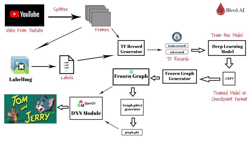
So first we’re going to see a complete end-to-end pipeline for training a custom object detector on our data and then we will use it in the OpenCV DNN module so we can get rid of the heavy Tensorflow framework for deployment. We have already discussed the advantages of using the final trained model in OpenCV instead of Tensorflow in my previous post.

Today’s post is the 3rd tutorial in our 3 part Deep Learning with OpenCV series. All three posts are titled as:

1. Deep Learning with OpenCV DNN Module, A Comprehensive Guide
2. Training a Custom Image Classifier with OpenCV, Converting to ONNX, and using it in OpenCV DNN module.
3. Training a Custom Object Detector with Tensorflow and using it with OpenCV DNN (This Post)

Now to follow along and to learn the full pipeline of training a custom object detector with TensorFlow you don’t need to read the previous two tutorials but when we move to the last part of this tutorial and use the model in OpenCV DNN then those tutorials would help.

What is Tensorflow Object Detection API (TFOD) :

To train our custom Object Detector we will be using TensorFlow API (TFOD API). The Tensorflow Object Detection API is a framework built on top of TensorFlow that makes it easy for you to train your own custom models.

The workflow generally goes like this :

You take a pre-trained model from this model zoo and then fine-tune the model for your own task.
Fine-tuning is a transfer learning method that allows you to utilize features of the model which it learned from a different task to your own task. Because of this, you won’t require thousands of images to train the network, only a few hundred will suffice.
If you’re someone who prefers PyTorch instead of Tensorflow then you may want to look at Detectron 2

For this Tutorial I will be using TensorFlow Object Detection API version 1, If you want to know why we are using version 1 instead of the recently released version 2, then you can read below optional explanation.

Tensorflow Object Detection API 1

Why we’re using Tensorflow Object Detection API Version 1? (OPTIONAL READ)

IGNORE THIS EXPLANATION IF YOU’RE NOT FAMILIAR WITH TENSORFLOW’S  FROZEN_GRAPHS

Tensorflow Object Detection API v2 comes with a lot of improvements, the new API contains some new State of The ART (SoTA) models, some pretty good changes including New binaries for train/eval/export that are eager mode compatible. You can check out this release blog from the Tensorflow Object Detection API developers.

But the thing is because TF 2 no longer supports sessions so you can’t easily export your model to frozen_inference_graph, furthermore TensorFlow depreciates the use of frozen_graphs and promotes saved_model format for future use cases.

For TensorFlow, this is the right move as the saved_model format is an excellent format.

So what’s the issue?

The problem is that OpenCV only works with frozen_inference_graphs and does not support saved_model format yet, so for this reason, if your end goal is to deploy it in OpenCV then you should use Tensorflow Object Detection API v1. Although you can still generate frozen_graphs, those graphs produce errors with OpenCV most of the time, we’ve tried limited experiments with TF2 so feel free to carry out your experiments but do share if you find something useful.

Now One great thing about this situation is that the Tensorflow team decided to keep the whole pipeline and code of Tensorflow Object Detection API 2 almost identical to Tensorflow Object Detection API 1 so learning how to use Tensorflow Object Detection API v1 will also teach you how to use Tensorflow Object Detection API v2.

Now Let’s start with the code

Code For TF Object Detection Pipeline:

[optin-monster slug=”qgtcyvbjr2wbqczjlxxm”]

Make sure to download the source code, which also contains the support folder with some helper files that you will need.

Here’s the hierarchy of the source code folder:

│   Colab Notebook Link.txt
│   Custom_Object_Detection.ipynb
│
└───support
    │   create_tf_record.py
    │   frozen_inference_graph.pb
    │   graph_ours.pbtxt
    │   tf_text_graph_common.py
    │   tf_text_graph_faster_rcnn.py
    │  
    │
    ├───labels
    │       _000.xml
    │       _001.xml
    │       _002.xml
    │       ...
    
    ├───test_images
    │       test1.jpg
    │       test2.jpg
    │       test3.png
    │       ...
    

Here’s a description of what these folders & files are:

• Custom_Object_Detection.ipynb: This is the main notebook which contains all the code.
• Colab Notebook Link: This text file contains the link for the colab version of the notebook.
• Create_tf_record.py: This file will create tf records from the images and labels.
• fronzen_graph_inference.pb: This is the model we trained, you can try to run this on test images.
• graph_ours.pbtxt: This is the graph file we generated for OpenCV, you’ll learn to generate your own.
• tf_text_graph_faster_rcnn.py: This file creates the above graph.pbtxt file for OpenCV.
• tf_text_graph_common.py: This is a helper file used by the faster_rcnnn.py file.
• labels: These are .xml labels for each image
• test_images: These are some sample test images to do inference on.

Note: There are some other folders and files which you will generate along the way, I will explain their use later.

Now Even though I make it really easy but still if you don’t want to worry about environment setup, installation, then you can use the colab version of the notebook that comes with the source code.

The Colab version doesn’t require any Configuration, It’s all set to go. Just run the cells in order. You should also be able to use the Colab GPU to speed up the training process.

The full code can be broken down into the following parts

• Part 1: Environment Setup
• Part 2: Installation & TFOD API Setup
• Part 3: Data Collection & Annotation
• Part 4: Downloading Model & Configuring it
• Part 5: Training and Exporting Inference Graph.
• Part 6: Generating .pbtxt and using the trained model with just OpenCV.

Part 1: Environment Setup:

First, let’s Make sure you have correctly set up your environment.

Since we are going to install TensorFlow version 1.15.0 so we should use a virtual environment, you can either install virtualenv or anaconda distribution. I’m using Anaconda. I will start by creating a virtual environment.

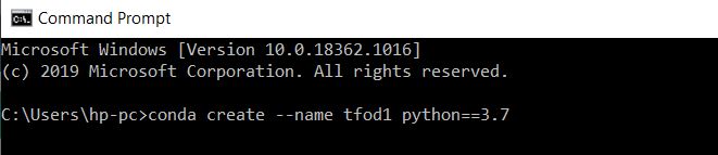
Open up the command prompt and do conda create --name tfod1 python==3.7

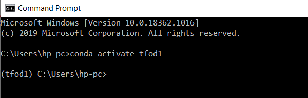
Now you can move into that environment by activating it:

conda activate tfod1

Make sure there is a (tfod1) at the beginning of each line in your cmd. This means you’re using that environment. Now anything you install will be in that environment and won’t affect your base/root environment.

The first thing You want to do is install a jupyter notebook in that environment. Otherwise, your environment will use the jupyter notebook of the base environment, so do:

pip install jupyter notebook

Now you should go into the directory/folder which I provided you and contains this notebook and open up the command prompt.

First, activate the environment tfod1 environment and then launch the jupyter notebook by typing jupyter notebook and hit enter.

This will launch the jupyter notebook in your newly created environment. You can now Open up Custom_Object_Detection Notebook.

Make sure your Notebook is Opened up in the Correct environment

import sys

# Make sure to check you're using your tfod1 environment, you should see that name in the printed output
print(sys.executable)

c:usershp-pcanaconda3envstfod1python.exe

Part 2: Installation & Tensorflow Object Detection API Setup: 

You can install all the required libraries by running this cell

# If you can't use ! on windows 10 then you should do conda install posix
# Alternatively you can also use % instead of ! in Windows.

!pip install tensorflow==1.15.0
!pip install youtube-dl
!pip install git+https://github.com/TahaAnwar/pafy.git#egg=pafy
!pip install scipy
!pip install labelImg
!pip install opencv-contrib-python
!pip install matplotlib

If you want to install Tensorflow-GPU for version 1 then you can take a look at my tutorial for that here

Note: You would need to change the Cuda Toolkit version and CuDNN version in the above tutorial since you’ll be installing for TF version 1 instead of version 2. You can look up the exact version requirements here

Another Library you will need is pycocotools

# RUN THIS TO INSTALL IN WINDOWS
!pip install pycocotools-windows

Alternatively, You can also use this command to install in windows:

pip install git+https://github.com/philferriere/cocoapi.git#egg=pycocotools^&subdirectory=PythonAPI

# RUN THIS TO INSTALL IN LINUX
pip install git+https://github.com/waleedka/cocoapi.git#egg=pycocotools&subdirectory=PythonAPI

Alternatively, you can also use this command to install in Linux and osx:

pip install pycocotools

Note: Make sure you have Cython installed first by doing: pip install Cython

Import Libraries

This will also confirm if your installations were successful or not.

import os
import shutil
import math
import datetime

import glob
import urllib
import tarfile
import urllib.request
from urllib.request import urlopen
from io import BytesIO
from zipfile import ZipFile
import re


import matplotlib.pyplot as plt
%matplotlib inline

# This will let you download any video from youtube
import pafy

import cv2
import numpy as np

import tensorflow as tf

print("This should be Version 1.15.0, DETECTED VERSION: " + tf.__version__)

This should be Version 1.15.0, DETECTED VERSION: 1.15.0

Clone Tensorflow Object Detection API Model Repository

You need to clone the TF Object Detection API repository, you can either download the zip file and extract it or if you have git installed then you can git clone it.

Option 1: Download with git:

You can run git clone if you have git installed, this is going to take a while, it’s 600 MB+, have a coffee or something.

# Clone the Github Repo in the current directory.
!git clone https://github.com/tensorflow/models.git

Option 2: Download the zip and extract all: (Only do this if you don’t have git)

You can download the zip by clicking here, after downloading make sure to extract the contents of this zip inside the directory containing this notebook. I’ve already provided you the code that automatically downloads and unzips the repo in this directory.

URL = 'https://github.com/tensorflow/models/archive/master.zip'

# Download and extract the zip file into a folder named support
with urlopen(URL) as zip_file:
    with ZipFile(BytesIO(zip_file.read())) as zfile:
        zfile.extractall()
        
# Rename `models-master` directory to `models`
os.rename('models-master', 'models')

The models we’ll be using are in the research directory of the above repo. The research directory contains a collection of research model implementations in TensorFlow 1 or 2 by researchers. There are a total of 4 directories in the above repo, you can learn more about them here.

Install Tensorflow Object Detection API & Compile Protos

Download Protobuff Compiler:

TFOD contains some files .proto format, I’ll explain more about this format in a later step, for now, you need to download the protobuf compiler from here, make sure to download the correct one based on your system. For e.g. I downloaded protoc-3.12.4-win64.zip for my 64-bit windows. For Linux and osx there are different files.

After downloading unzip the proto folder, go to its bin directory, and copy the proto.exe file. Now paste this proto.exe inside the models/research directory.

The below script does all of this, but you can choose to do it manually if you want. Make sure to change the URL if you’re using a system other than 64-bit windows.

# Set the URL, you can copy/paste your target system's URL here.
URL = 'http://github.com/protocolbuffers/protobuf/releases/download/v3.12.4/protoc-3.12.4-win64.zip'

name = 'proto_file'

# Download and extract the zip file into a folder named proto_file
with urlopen(URL) as zip_file:
    with ZipFile(BytesIO(zip_file.read())) as zfile:
        zfile.extractall('proto_file')
        
# Copy and paste the protoc.exe to 'models/research' directory.
shutil.copy(name + '/bin/protoc.exe', 'models/research/')   

# Delete the protoc folder
shutil.rmtree(name)

Now you can install the object detection API and compile the protos:
Below two operations must be performed in this directory, otherwise, it won’t work, especially the proto command.

# Move to models/research directory.
os.chdir('models/research/')

# Compiles protobuf files in the object_detction/protos folder, Now for every .proto there will be .py file present there.
!protoc object_detectionprotos*.proto --python_out=.

# Copies the requied setup file
!cp object_detection/packages/tf1/setup.py .

# Installs and setsup TF 1 Object Detection API.
!python -m pip install .

# Move up two directories, this will put you back to your original `TF Object Detection v1` directory.
os.chdir('../..')

Note: Since I already had installed pycocotools so after running this line cp object_detection/packages/tf1/setup.py . I edited the setup.py file to get rid of pycocotools package inside the REQUIRED_PACKAGES list then I saved the setup.py file and ran the python -m pip install . command. I did this because I was facing issues installing pycocotools this way which is why I installed the pycocotools-windows package, you probably won’t need to do this.

If you wanted to install TFOD API version 2 instead of version 1 then you can just replace tf1 with tf2 in the cp object_detection/packages/tf1/setup.py . command.

You can check your installation of TFOD API by running model_builder_tf1_test.py

# Move to models/research directory.
os.chdir('models/research/')

# Test the installation.
!python object_detection/builders/model_builder_tf1_test.py

# back to the main directory
os.chdir('../..')

Part 3: Data Collection & Annotation:

Now for this tutorial, I’m going to train a detector to detect the faces of Tom & Jerry. I didn’t want to use the common animal datasets etc. So I went with this.

While I was writing the above sentence I just realized I’m still using a Cat, mouse dataset albeit an animated one so I guess it’s still a unique dataset.

In this tutorial, I’m not only going to show you how to annotate the data but also show you one approach on how to go about collecting data for a new problem.

So What I’ll be doing is that I’m going to download a video of Tom & Jerry from Youtube and then split the frames of the video to create my dataset and then annotate each of those frames with bounding boxes. Now instead of downloading my Tom & Jerry video you can use any other video and try to detect your own classes.

Alternatively, you can also generate training data from other methods including getting images from Google Images.

To prepare the Data we need to perform these 5 steps:

• Step 1: Download Youtube Video.
• Step 2: Split Video Frames and store it.
• Step 3: Annotate Images with labelImg.
• Step 4: Create a label Map file.
• Step 5: Generate TFRecords.

Step 1: Download Youtube Video:

# Define the URL of the video
url = "https://www.youtube.com/watch?v=blWvD93bALE"

# Set the name of the Video 
video_name =  "support/test_images/tomandjerry.mp4"

# Create video object
video = pafy.new(url)

# Get that video in best available resolution
bestResolutionVideo = video.getbest()

# Download the Video
bestResolutionVideo.download(filepath= video_name)

11,311,502.0 Bytes [100.00%] received. Rate: [7788 KB/s]. ETA: [0 secs]

For more options on how you can download the video take a look at the documentation here

Step 2: Split Video Frames and store it:

Now we’re going to split the video frames and store them in a folder. Since most videos have a high FPS (30-60 frames/sec) and we don’t exactly need this many frames for two reasons:

1. If you take a 30 FPS video then for each second of the video you will get 30 images and most of those images won’t be different from each other, there will be a lot of repetition of information.
2. We’re already going to use Transfer Learning with TFOD API, the benefit of this is that we won’t be needing a lot of images and this is good since we don’t want to annotate thousands of images.

So we can do two things we can skip frames and save every nth frame or we can save a frame every nth second of the video. I’m going with the latter approach, although both are valid approaches.

# Define an output directory
output_directory = "training/images"

# Define the time interval after which you'll save each frame.
sec = 1.5

# If the output directory does not exists then create it
if not os.path.exists(output_directory):
    os.makedirs(output_directory)

# Initialize the video capture object
cap = cv2.VideoCapture(video_name)

# Get the FPS rate of the video, for this video its 25.0
fps = cap.get(cv2.CAP_PROP_FPS)

# Given the FPS rate of the video calculate the no of frames you will need to skip to determine that `sec` seconds are passed.
no_of_frames_to_skip = round(sec * fps)

frame_count = 0

while True:

    ret, frame = cap.read()
    
    # Break the loop if the video has ended
    if not ret:
        break

    # Get the Current Frame Number
    frame_Id = int(cap.get(1))

    # Only Save the frame when you've skipped the defined the number of frames
    if frame_Id % no_of_frames_to_skip == 0:
        
        # Save the frame in the output directory
        #fname = "n_{}.jpg".format(frame_count)
        fname = '_{str_0:0>{str_1}}.jpg'.format(str_0=frame_count, str_1=3)
        cv2.imwrite(os.path.join(output_directory, fname), frame)

        frame_count += 1
        
print('Done Splitting Video, Total Images saved: {}'.format(frame_count))

# Release the capture
cap.release()

Done Splitting Video, Total Images saved: 165

You can go to the directory where the images are saved and manually go through each image and delete the ones where Tom & Jerry are not visible or hardly visible. Although this is not a strict requirement since you can easily skip these images in the annotation step.

Step 3: Annotate Images with labelImg

You can watch this video below to understand how to use labelImg to annotate images and export annotations. You can also take a look at the GitHub repo here.

For the current Tom & Jerry problem, I am providing you with a labels folder that already contains the .xml annotation file for each image. If you want to try a different dataset then go ahead, make sure to put the labels of that dataset in the labels folder

Note: We are not splitting the images into the train and validation folder right now because we’ll be doing that automatically at tfrecord creation step. Although it would still be a good idea to separate 10% of the data for proper testing/evaluation of the final trained detector, since my purpose is to make this tutorial as simple as possible so I won’t be doing that today, I already have test folder with 4-5 images which I will evaluate on.

Step 4: Create a label Map file

TensorFlow requires a label map file, which maps each of the class labels to integer values. This label map is used in the training and detection process. This file should be saved in training the directory which also contains the labels folder

# You can add more classes by adding another item and giving them an id of 3 and so on.

pbtxt = '''

item {
    id: 1
    name: 'Jerry'
}

item {
    id: 2
    name: 'Tom'
}

'''

with open("training/label_map.pbtxt", "w") as text_file:
    text_file.write(pbtxt)

Step 5: Generate TFrecords

What are TFrecords?

Tfrecords are just protocol buffers, they help make the data reading/processing process computationally efficient. The only downside they have is that they are not human-readable.

What are protocol Buffers?

A protocol buffer is a type of serialized structured data. It is more efficient than JSON, XML, pickle, and text storage formats. Google created this Protobuf (protocol buffer) format in 2008 because of their efficiency, Since then they have been widely used by Google and the community. To read the protobuf files (.proto files) you will first need to compile them by a protobuf compiler. So now you probably understand why we needed to compile those proto files at the beginning.

Here’s a nice tutorial by Naveen that explains how you can create a tfrecord for different data types and Here’s a more detailed explanation of protocol buffers with an example.

The create_tf_record.py script I’ll be using to convert images/labels to tfrecords is taken from the TensorFlow’s pet example but I’ve modified the script so now it accepts the following 5 arguments:

1. Directory of images
2. Directory of labels
3. % of Split of Training data
4. Path to label_map.pbtxt file
5. Path to output tfrecord files

And it returns a train.record and val.record. So it splits the training data into training/validation sets. For this data, I’m using a training set of 70% and validation is 30%.

# Create tfrecords directory if it does not exits. This is where tfrecords will be stored.
tf_reocords = "training/tfrecords"
if not os.path.exists(tf_reocords):
    os.mkdir(tf_reocords)

# We are saving the record files in the folder named tfrecords.
# Change the slashes (i.e. ) according to your OS system.
# I'm using my own labels you can replace them with your labels.
!python supportcreate_tf_record.py --image_dir trainingimages --split 0.7 --labels supportlabels   
--output_path trainingtfrecords --label_map  traininglabel_map.pbtxt

Done Writing, Saved: trainingtfrecordstrain.record Done Writing, Saved: trainingtfrecordsval.record

You can ignore these warnings, we already know that we’re using an older 1.15 version of TFOD API which contains some depreciated functions.

Most of the tfrecord scripts available online will first tell you to convert your xml files to csv and then you will use another script to split the data into a training and validation folder and then another script to convert to tfrecords. The script above is doing all of this.

Part 4: Downloading Model & Configuring it:

You can now go to the Model Zoo, select a model, and download its zip. Now unzip the contents of that folder and put them inside a directory named pretrained_model. The below script does this automatically for a Faster-RCNN-Inception model which is already trained on the COCO dataset. You can change the model name to download a different model.

# Specify pre-trained model name you want to download
MODEL = 'faster_rcnn_inception_v2_coco_2018_01_28'

# Add the zip extension to the model
MODEL_FILE = MODEL + '.tar.gz'

# Define the base URL
DOWNLOAD_BASE = 'http://download.tensorflow.org/models/object_detection/'

# If model directory is present then remove if for the new model
model_directory = "pretrained_model"
if os.path.exists(model_directory):
    shutil.rmtree(model_directory )

# Download the pretrained Model
opener = urllib.request.URLopener()
opener.retrieve(DOWNLOAD_BASE + MODEL_FILE, MODEL_FILE)

# Here we are extracting the downloaded file
tar = tarfile.open(MODEL_FILE)
tar.extractall()
tar.close()

# Removing the downloaded zip file.
os.remove(MODEL_FILE)

# Rename model directory to pretrained_model
os.rename(MODEL, model_directory)

# Remove the checkpoint file so the model can be trained
os.remove(model_directory + '/checkpoint')

print('Model Downloaded')

Model Downloaded

Modify pipline.config file:

After downloading you will have a number of files present in the pretrained_model folder, I will explain about them later but for now, let’s take a look at the pipeline.config file.

Pipeline.config defines how the whole training process will take place, what optimizers, loss, learning_rate, batch_size will be used. Most of these params are already set by default, it’s up to you if you want to change them or not but there are some paths in the pipeline.config file that you will need to change so that this model can be trained on our data.

So open up pipeline.config with a text editor like Notepad ++ and change these 4 paths:

• Change: PATH_TO_BE_CONFIGURED/model.ckpt  to  pretrained_model/model.ckpt
• Change: PATH_TO_BE_CONFIGURED/mscoco_train.record  to  training/tfrecords/train.record
• Change: PATH_TO_BE_CONFIGURED/mscoco_val.record   to  training/tfrecords/val.record
• Change: PATH_TO_BE_CONFIGURED/mscoco_label_map.pbtxt  to  training/label_map.pbtxt
• Change: num_classes: 90  to  num_classes: 2

If you’re lazy like me then no prob, below script does all this

# Path of pipeline configuration file
filename = model_directory + '/pipeline.config'

# Open the configutation file and read the whole file
with open(filename) as f:
    s = f.read()
    
# Now find and subsitute the source paths with the destinations paths.    
with open(filename, 'w') as f:
    s = re.sub('PATH_TO_BE_CONFIGURED/model.ckpt', model_directory + '/model.ckpt', s)
    s = re.sub('PATH_TO_BE_CONFIGURED/mscoco_train.record', 'training/tfrecords/train.record', s)
    s = re.sub('PATH_TO_BE_CONFIGURED/mscoco_val.record', 'training/tfrecords/val.record', s)
    s = re.sub('PATH_TO_BE_CONFIGURED/mscoco_label_map.pbtxt', 'training/label_map.pbtxt', s)
    
    # Since we have 2 classes (Tom, Jerry) so we set this value to 2.
    s = re.sub('num_classes: 90', 'num_classes: 2', s)

    
    # Doing a little correction to avoid an error in training.
    s = re.sub('step: 0', 'step: 1', s)
            
    # I'm also changing the default batch_size of 1 to be 10 for this example
    s = re.sub('batch_size: 1', 'batch_size: 10', s)
    f.write(s)

Notice the correction I did by replacing step: 0 with step: 1, unfortunately for different models sometimes there are some corrections required but you can easily understand what exactly needs to be changed by pasting the error generated during training on google. Click on GitHub issues for that error and you’ll find a solution for that.

Note: These issues seem to be mostly present in TFOD API Version 1

Changing Important Params in Pipeline.config File:

Additionally, I’ve also changed the batch size of the model, just like batch_size, there are lots of important parameters that you would want to tune. I would strongly recommend that you try to change the values according to your problem. Almost always the default values are not optimal for your custom use case. I should tell you that to tune most of these values you need some prior knowledge, make sure to at least change the batch_size according to your system’s memory and learning_rate of the model.

Part 5 Training and Exporting Inference Graph: 

You can start training the model by calling the model_main.py script from the Object_detection folder, we are giving it the following arguments.

• num_train_steps: These are the number of times your model weights will be updated using a batch of data.
• pipeline_config_path: This is the path to your pipeline.config file.
• model_dir: Path to the output directory where the final checkpoint files will be saved.

Now you can run the below cell to start training but I would recommend that you run this cell in the command line, you can just paste this line:

# Start Training
!python models/research/object_detection/model_main.py  --pipeline_config_path="pretrained_modelpipeline.config" 
--model_dir="pretrained_model"  --num_train_steps=20000 

Note: When you start training you will see a lot of warnings, just ignore them as TFOD 1 contains a lot of deprecated functions.

Once you start training, the network will take some time to initialize and then the training will start, after every few minutes, you will see a report of loss values and a global loss. The Network is learning if the loss is going down. If you’re not familiar with the Object detection Jargon Like IOU etc, then just make note of the final global loss after each report.

You ideally want to set the num_train_steps to tens of thousands of steps, you can always end training by pressing CTRL + C on the command prompt if the loss has decreased sufficiently. If training is taking place in jupyter notebook then you can end it by pressing the Stop button on top.

After training has ended or you’ve stopped it, there would be some new files in the pre_trained folder. Among all these files we will only need the checkpoint (ckpt) files.

If you’re training for 1000s of steps (which is most likely the case) then I would strongly recommend that you don’t use your CPU but utilize a GPU. If you don’t have one then it’s best to use Google Colab’s GPU. I’m already providing you a ready-to-run colab Notebook.

Note: There’s another script for training called train.py, this is an older script where you can see the loss value for each step, if you want to use that script then you can find it at models / research / object_detection / legacy / train.py

You can run this script by doing:

python models/research/object_detection/legacy/train.py --pipeline_config_path="pretrained_modelpipeline.config" 
--train_dir="pretrained_model"

The best way to monitor training is to use Tensorboard, I will discuss this another time

Export Frozen Inference Graph:

Now we will use the export_inference_graph.py script to create a frozen_inference_graph from the checkpoint files.

Why are we doing this?

After training our model it is stored in checkpoint format and a saved_model format but in OpenCV, we need the model to be in a frozen_inference_graph format. So we need to generate the frozen_inference_graph using the checkpoint files.

What are these checkpoint files?

After Every few minutes of training, TensorFlow outputs some checkpoint (ckpt) files. The number on those files represents how many train steps they have gone through. So during the frozen_inference_graph creation, we only take the latest checkpoint file (i.e. the file with the highest number) because this is the one that has gone through the most training steps.

Now every time a checkpoint file is saved, it’s split into 3 parts.

For the initial step these files are:

• model.ckpt-000.data: This file contains the value of each single variable, its pretty large.
• model.ckpt-000.info: This file contains metadata for each tensor. e.g. checksum, auxiliary data etc.
• model.ckpt-000.meta: This file stores the graph structure of the model

# Get all the files present in the pretrained_model directory
lst = os.listdir(model_directory)

# Get the most recent checkpoint file number.
lf = filter(lambda k: 'model.ckpt-' in k, lst)
check = sorted([int(x.split('ckpt-')[1].split('.')[0]) for x in sorted(lf)[:]])[-1]

# Attach that number to model.ckpt- and pass it to the export script.
checkpoint = 'model.ckpt-' + str(check)

# Run the export script, it takes the input_type, pipeline.config path,latest checpoint file name and  output path  
!python modelsresearchobject_detectionexport_inference_graph.py  
--input_type image_tensor 
--pipeline_config_path pretrained_model/pipeline.config  
--trained_checkpoint_prefix pretrained_model/$checkpoint 
--output_directory fine_tuned_model

If you take a look at the fine_tuned_model folder which will be created after running the above command then you’ll find that it contains the same files you got when you downloaded the pre_trained model. This is the final folder.

Now Your trained model is in 3 different formats, the saved_model format, the frozen_inference_graph format, and the checkpoint file format. For OpenCV, we only need the frozen inference graph format.

The checkpoint format is ideal for retraining purposes and getting to know other sorts of information about the model, for production and serving the model you will need to use is either the frozen_inference_graph or saved_model format. It’s worth mentioning that both these files contain the extension .pb

In TF 2, frozen_inference_graph is depreciated and TF 2 encourages to use the saved_model format, as said previously unfortunately we can’t use the saved_model format with OpenCV yet.

Run Inference on Trained Model (Bonus Step):

You can optionally choose to run inference using TensorFlow sessions, I’m not going to explain much here as Tf sessions are depreciated and our final goal is to actually use this model in OpenCV DNN.

frozen_graph_path = 'fine_tuned_model/frozen_inference_graph.pb'

#0.49179258942604065

# Read the graph.
with tf.gfile.FastGFile(frozen_graph_path, 'rb') as f:
    graph_def = tf.GraphDef()
    graph_def.ParseFromString(f.read())

with tf.Session() as sess:
    
    # Set the defualt session
    sess.graph.as_default()
    tf.import_graph_def(graph_def, name='')

    # Read the Image
    img = cv2.imread('support/test_images/test7.jpg')
    
    # Get the rows and cols of the image.
    rows = img.shape[0]
    cols = img.shape[1]
    
    # Resize the image to 300x300, this is the size the model was trained on
 
    inp = cv2.resize(img, (300, 300))
    
    # Convert OpenCV's BGR image to RGB
    inp = inp[:, :, [2, 1, 0]]  # BGR2RGB

    # Run the model
    out = sess.run([sess.graph.get_tensor_by_name('num_detections:0'),
                    sess.graph.get_tensor_by_name('detection_scores:0'),
                    sess.graph.get_tensor_by_name('detection_boxes:0'),
                    sess.graph.get_tensor_by_name('detection_classes:0')],
                   feed_dict={'image_tensor:0': inp.reshape(1, inp.shape[0], inp.shape[1], 3)})

    # These are the classes which we want to detect
    classes = {1: "Jerry", 2: 'Tom'}
    
    # Get the total number of Detections
    num_detections = int(out[0][0])
    
    # Loop for each detection
    for i in range(num_detections):
        
        # Get the probability of that class
        score = float(out[1][0][i])
        
        # Check if the score of the detection is big enough
        if score > 0.400:
                                
            # Get their Class ID
            classId = int(out[3][0][i])

            # Get the bounding box coordinates of that class
            bbox = [float(v) for v in out[2][0][i]]
            
            # Get the class name
            class_name = classes[classId]
            
            # Get the actual bounding box coordinates
            x = int(bbox[1] * cols)
            y = int(bbox[0] * rows)
            right = int(bbox[3] * cols)
            bottom = int(bbox[2] * rows)
            
            # Show the class name and the confidence
            cv2.putText(img, "{} {.:2f}%".format(class_name, score*100), x, bottom+30, cv2.FONT_HERSHEY_SIMPLEX, 1, (255,0,255), 4)
            
            # Draw the bounding box
            cv2.rectangle(img, x, y, right, bottom, (125, 255, 51), thickness = 2)

# Show the image with matplotlib           
plt.figure(figsize=(10,10))
plt.imshow(img[:,:,::-1]);

Part 6: Generating .pbtxt and using the trained model with just OpenCV 

6 a) Export Graph.pbxt with frozen inference graph:

We can use the above generated frozen graph inside the OpenCV DNN module to do detection but most of the time we need another file called a graph.pbtxt file. This file contains a description of the network architecture, it is required by OpenCV to rewire some network layers for Optimization purposes.

This graph.pbtxt can be generated by using one of the 4 scripts provided by OpenCV. These scripts are:

• tf_text_graph_ssd.py
• tf_text_graph_faster_rcnn.py
• tf_text_graph_mask_rcnn.py
• tf_text_graph_efficientdet.py

They can be downloaded here, you will also find more information regarding them on that page.

Now since the Detection architecture we’re using is Faster-RCNN (you can tell by looking at the name of the downloaded model) so we will use tf_text_graph_faster_rcnn.py to generate the pbtxt file. For .pbtxt generation you will need the frozen_inference_graph.pb file and the pipeline.config file.

Note: When you’re done with training then you will also see a graph.pbtxt file inside the pretrained folder, this graph.pbtxt is different from the one generated by OpenCV’s .pbtxt generator scripts. One major difference is that the OpenCV’s graph.pbtxt do not contain the model weights but only contain the graph description, so they will be much smaller in size.

!python support/tf_text_graph_faster_rcnn.py --input "fine_tuned_model/frozen_inference_graph.pb" 
--config "pretrained_model/pipeline.config" --output "support/graph.pbtxt"

Number of classes: 2
Scales: [0.25, 0.5, 1.0, 2.0] Aspect ratios: [0.5, 1.0, 2.0]
Width stride: 16.000000
Height stride: 16.000000
Features stride: 16.000000

For model architectures that are not one of the above 4, then for those, you will need to convert TensorFlow’s .pbtxt file to OpenCV’s version. You can find more on how to do that here. But we warned this conversion is not a smooth process and there are a lot of low-level issues that come up.

6 b) Using the Frozen inference graph along with Pbtxt file in OpenCV:

Now that we have generated the graph.pbtxt file with OpenCV’s tf_text_graph function we can pass this file to cv2.dnn.readNetFromTensorflow() to initialize the network. All of our work is done now Make sure you’re familiar with OpenCV’s DNN module, if not you can read my previous post on it.

Now we will create the following two functions:

Initialization Function: This function will initialize the network using the .pb and .pbtxt files, it will also set the class labels.

Main Function: This function will contain all the rest of the code from preprocessing to postprocessing, it will also have the option to either return the image or display it with matplotlib

# We're passing in the paths of pbtxt file (graph description of model) and our actual trained model

def initialize(pbtxt = 'support/graph.pbtxt', model = "fine_tuned_model/frozen_inference_graph.pb" ):
    
    # Define global variables
    global net, classes

    # ReadNet function takes both files and intitialize the network
    net = cv2.dnn.readNetFromTensorflow(model, pbtxt);

    # Define Class Labels
    classes = {0: "Jerry", 1: 'Tom'}

This is our main function, the comments will explain what’s going on

def detect_object(img, returndata=False, conf = 0.9):
    
    # Get the rows, cols of Image 
    rows, cols, channels = img.shape

    # This is where we pre-process the image, Resize the image and Swap Image Channels
    # We're converting BGR channels to RGB since OpenCV reads in BGR and our model was trained on RGB images
    blob = cv2.dnn.blobFromImage(img, size=(300, 300), swapRB=True)
    
    # Set the blob as input to the network
    net.setInput(blob)

    # Runs a forward pass, this is where the model predicts on the image.
    networkOutputs = net.forward()

    # Loop over the output results
    for detection in networkOutputs[0,0]:
        
        # Get the score for each detection
        score = float(detection[2])
        
        # IF the class score is bigger than our threshold
        if score > conf:
            
            # Get the index of the class i.e. 1 or 2
            class_index = int(detection[1])
            
            # Use the Class index to get the class name i.e. Jerry or tom
            class_name = classes[class_index]
            
            # Get the bounding box coordinates.
            # Note: the returned coordinates are relative e.g. they are in 0-1 range.
            # Se we multiply them by rows and cols to get the real coordinates.
            x1 = int(detection[3] * cols)
            y1 = int(detection[4] * rows)
            x2 = int(detection[5] * cols)
            y2 = int(detection[6] * rows)
            
            # Show the class name and the confidence
            text = "{},  {:.2f}% ".format(class_name, score*100)
            cv2.putText(img, text, (x1, y2+ 30), cv2.FONT_HERSHEY_SIMPLEX, 0.6, 
                        (255,0,255), 2)
            
            # Draw the bounding box
            cv2.rectangle(img, (x1, y1), (x2, y2), (125, 255, 51), thickness = 2)

    # Return the annotated image if returndata is True
    if  returndata:
        return img
    
    # Otherwise show the full image.
    else:
        plt.figure(figsize=(10,10))
        plt.imshow(img[:,:,::-1]);plt.axis("off");                      

Note: When you do net.forward() you get an output of shape (1,1,100,7). Since we’re predicting on a single image instead of a batch of images so you will get (1,1) at the start now the remaining (100,7) means that there are 100 detections for that image and each image contains 7 properties/variables.

There will be 100 detections for each image, this was set in the pipeline.config, you can choose to change that.

So here are what these 7 properties correspond to:

1. This is the index of image for a single image its 0
2. This is the index of the target CLASS
3. This is the score/confidence of that CLASS

Remaining 4 values are x1,y1,x2,y2. These are used to draw the bounding box of that CLASS object

4. x1
5. y1
6. x2
7. y2

Initialize the network

You will just need to call this once to initialize the network

# You can initialize the model using our provided trained model
initialize()

# Or use your own trained model
initialize(pbtxt = 'support/graph.pbtxt', model = 'fine_tuned_model/frozen_inference_graph.pb' )

Predict On Images

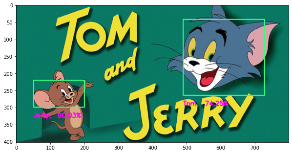
Now you can use the main function to perform prediction on different images, The images we will predict are placed inside a folder named test_images. These images were not in the training dataset.

img = cv2.imread('support/test_images/test1.jpg')
detect_object(img)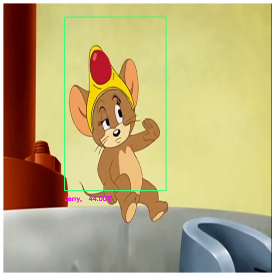

img = cv2.imread('support/test_images/test2.jpg')
detect_object(img)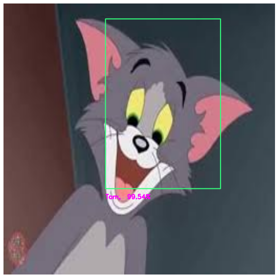

img = cv2.imread('support/test_images/test6.jpg')
detect_object(img)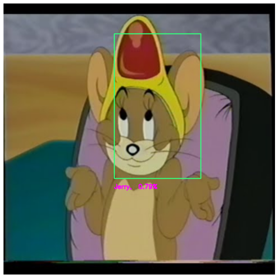

img = cv2.imread('support/test_images/test3.png')
detect_object(img)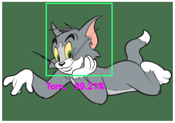

img = cv2.imread('support/test_images/test7.jpg')
detect_object(img)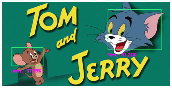

Summary

Limitations: Our Final detector has a decent accuracy but it’s not that robust because of 4 reasons:

1. Transfer Learning works best when the dataset you’re training on shares some features with the original dataset it was trained on, most of the models are trained on ImageNet, COCO, PASCAL VOC datasets. Which is filled with animals and other real-world images. Now our dataset is a dataset of Cartoon images, which is drastically different from real-world images. We can solve this problem by including more images and training more layers of the model.
   
   
2. Animations of cartoon characters are not consistent, they change a lot in different movies. So if you train the model on these pictures and then try to detect random google images of tom and jerry then you won’t get good accuracy. We can solve this problem by including images of these characters from different movies so the model learns the features that are the same throughout the movies.
   
   
3. The images generated from the sample video created an imbalanced dataset, There are more Jerry Images than Tom images, there are ways to handle this scenario but try to get a decent balance of images for both classes to get the best results.
   
   
4. The annotation is poor, Yeah so the annotation I did was just for the sake of making this tutorial, in reality, you want to set a clear outline and standard about how you’ll be annotating, are you going to annotate the whole head, are ears included, is the neck part of it.. so you need answer all these questions ahead of time.

I will stress again that if you’re not planning to use OpenCV for the final deployment then use TFOD API version 2, it’s a lot more cleaner. However, if the final objective is to use OpenCV at the end then you could get away with TF 2 but it’s a lot of trouble.

Even with TFOD API v1, you can’t be sure that your custom trained model will always be loaded in OpenCV correctly, there are times when you would need to manually edit the graph.pbtxt file so that you can use the model in OpenCV. If this happens and you’re sure you have done everything correctly then your best bet is to raise an issue here.

Hopefully, OpenCV will catch up and start supporting TF 2 saved_model format but it’s gonna take time. If you enjoyed this tutorial then please feel free to comment and I’ll gladly answer you.

You can reach out to me personally for a 1 on 1 consultation session in AI/computer vision regarding your project. Our talented team of vision engineers will help you every step of the way. Get on a call with me directly here.