In the previous tutorial we learned how the DNN module in OpenCV works, we went into a lot of details regarding different aspects of the module including where to get the models, how to configure them, etc. 

This Tutorial will build on top of the previous one so if you haven’t read the previous post then you can read that here. 

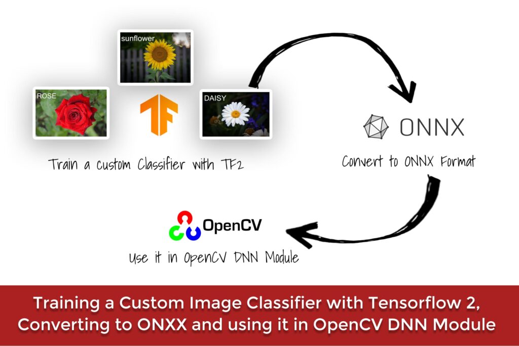
Today’s post is the second tutorial in our brand new 3 part Deep Learning with OpenCV series. All three posts are titled as:

1. Deep Learning with OpenCV DNN Module, A Comprehensive Guide
2. Training a Custom Image Classifier with OpenCV, Converting to ONNX, and using it in the OpenCV DNN module.
3. Using a Custom Trained Object Detector with OpenCV DNN Module.

In this post, we will train a custom image classifier with Tensorflow’s Keras API. So if you want to learn how to get started creating a Convolutional Neural Network using Tensorflow, then this post is for you, and not only that but afterward, we will also convert our trained .h5 model to ONNX format and then use it with OpenCV DNN module.

Converting your model to onnx will give you more than a 3x reduction in model size.

This whole process shows you how to train models in Tensorflow and then deploy them directly in OpenCV.

What’s the advantage of using the trained model in OpenCV vs using it in Tensorflow?

So here are some points you may want to consider.

• By using OpenCV’s DNN module, the final code is a lot compact and simpler.
  
• Someone who’s not familiar with the training framework like TensorFlow can also use this model.
  
• There are cases where using OpenCV’s DNN module will give you faster inference results for the CPU. See these results in LearnOpenCV by Satya.
  
• Besides supporting CUDA based NVIDIA’s GPU, OpenCV’s DNN module also supports OpenCL based Intel GPUs.
  
• Most Importantly by getting rid of the training framework (Tensorflow) not only makes the code simpler but it ultimately gets rid of a whole framework, this means you don’t have to build your final application with a heavy framework like TensorFlow. This is a huge advantage when you’re trying to deploy on a resource-constrained edge device, e.g. a Raspberry pie

So this way you’re getting the best of both worlds, a framework like Tensorflow for training and OpenCV DNN for faster inference during deployment.

This tutorial can be split into 3 parts.

1. Training a Custom Image Classifier in OpenCV with Tensorflow
2. Converting Our Classifier to ONNX format.
3. Using the ONNX model directly in the OpenCV DNN module.

Let’s start with the Code

Download Code

[optin-monster slug=”scb99lhehb40udr0ckhj”]

Part 1: Training a Custom Image Classifier with Tensorflow:

For this tutorial you need OpenCV 4.0.0.21 and Tensorflow 2.2

So you should do:

pip install opencv-contrib-python==4.0.0.21
(Or install from Source, Make sure to change the version)

pip install tensorflow
(Or install tensorflow-gpu from source)

Note: The reason I’m asking you to install version 4.0 instead of the latest 4.3 version of OpenCV is that later on, we’ll be using a function called readNetFromONNX() now with our model this function was giving an error in 4.3 and 4.2, possibly due to some bug in those versions. This does not mean that you can’t use custom models with those versions but that for my specific case there was an issue. Converting models only takes 2-3 lines of code but sometimes you get ambiguous errors that are hard to diagnose, but it can be done.

Hopefully, the conversion process will get better in the future.

One thing you can do is create a custom environment (with Anaconda or virtualenv) in which you can install version 4.0 without affecting your root environment and if you’re using google colab for this tutorial then you don’t need to worry about that.

You can go ahead and download the source code from the download code section. After downloading the zip folder, unzip it and you will have the following directory structure.

Flower_Classifier
    │   Custom Image Classifier .ipynb
    │
    ├───Images
    │       daisy.jpg
    │       daisy1.jpg
    │       dandelion.jpg
    │       rose.jpg
    │       sunflower.jpg
    │       tulip.jpg
    │
    └───Model
            flowers.h5
            flowers_model.onnx

You can start by importing the libraries:

# Import Required libraries
import tensorflow as tf
from tensorflow.keras.models import Sequential, load_model, Model
from tensorflow.keras.layers import Dense, Conv2D, Dropout, MaxPooling2D, GlobalAveragePooling2D, Activation
from tensorflow.keras.preprocessing.image import ImageDataGenerator
from tensorflow.keras.optimizers import Adam
import os
import numpy as np
import cv2
import matplotlib.pyplot as plt
import urllib.request
import tarfile

Let’s see how you would go about training a basic Convolutional Network in Tensorflow. I assume you know some basics of deep learning. Also in this tutorial, I will be teaching how to construct and train a classifier using a real-world dataset, not a toy one, I will not go in-depth and explain the theory behind neural networks. If you want to start learning deep learning then you can take a look at Andrew Ng’s Deep Learning specialization, although this specialization is basic and covers mostly foundational things now if your end goal is to specialize in computer Vision then I would strongly recommend that you first learn Image Processing and Classical Computer Vision techniques from my 3-month comprehensive course here.

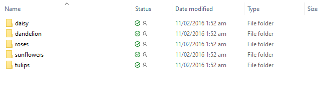
The Dataset we’re going to use here is a dataset of 5 different flowers, namely rose, tulips, sunflower, daisy, and dandelion. I avoided the usual cats and dogs dataset.

You can download the dataset from a URL, you just have to run this cell

url = ' https://storage.googleapis.com/download.tensorflow.org/example_images/flower_photos.tgz'
filename = 'flower_photos.tgz'
urllib.request.urlretrieve(url, filename)

After downloading the dataset you’ll have to unzip it, you can also do this manually.

filename = "flower_photos.tgz"
tf = tarfile.open(filename)
tf.extractall()

After extracting you can check the folder named flower_photos in your current directory which will contain these 5 subfolders.

You can check the number of images in each class using the code below.

# This is the directory path where all the class folders are
dir_path =  'flower_photos'

# Initialize classes list, this list will contain the names of our classes.
classes = []

# Iterate over the names of each class
for class_name in os.listdir(dir_path):

   # Get the full path of each class
  class_path = os.path.join(dir_path, class_name)
  
  # Check if the class is a directory/folder
  if os.path.isdir(class_path):

      # Get the number of images in each class and print them
      No_of_images = len(os.listdir(class_path))
      print("Found {} images of {}".format(No_of_images , class_name))

      # Also store the name of each class
      classes.append(class_name)

# Sort the list in alphabatical order and print it    
classes.sort()
print(classes)

Found 699 images of sunflowers
Found 898 images of dandelion
Found 633 images of daisy
Found 799 images of tulips
Found 641 images of roses
[‘daisy’, ‘dandelion’, ‘roses’, ‘sunflowers’, ‘tulips’]

Generate Images:

Now it’s time to load up the data, now since the data is approx 218 MB, we can actually load it in RAM but most real datasets are large several GBs in size, and will fit in your RAM. In those scenarios, you use data generators to fetch batches of data and feed it to the neural network during training, so today we’ll also be using a data generator to load the data.

Before we can pass the images to a deep learning model, we need to do some preprocessing, like resizing the image in the required shape, converting them to floating-point tensors, rescale the pixel values from 0-255 to 0-1 range as this helps in training.

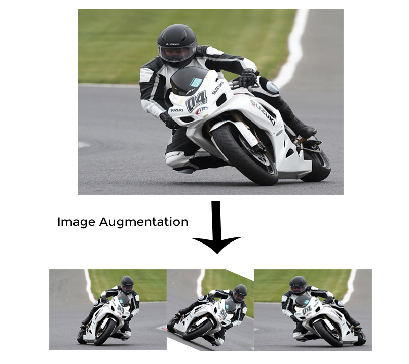
Fortunately, all of this can be done by the ImageDataGenerator class in tf.keras. Not only that but the ImageDataGenerator Class can also perform data augmentation. Data augmentation means that the generator takes your image and performs random transformations like randomly rotating, zooming, translating, and performing other such operations to the image. This is really effective when you don’t have much data as this increases your dataset size on the fly and your dataset contains more variation which helps in generalization.

As you’ve already seen that each flower class has less than 1000 examples, so in our case data augmentation will help a lot. It will expand our dataset.

When training a Neural Network, we normally use 2 datasets, a training dataset, and a validation dataset. The neural network tunes its parameters using the training dataset and the validation dataset is used for the evaluation of the Network’s performance.

# Set the batch size, width, height and the percentage of the validation split.
batch_size = 60
IMG_HEIGHT = 224
IMG_WIDTH = 224
split = 0.2


#  Setup the ImagedataGenerator for training, pass in any supported augmentation schemes, notice that we're also splitting the data with split argument.
datagen_train = tf.keras.preprocessing.image.ImageDataGenerator(
    rescale=1./255, 
    validation_split= split,
    rotation_range=20,
    width_shift_range=0.1,
    height_shift_range=0.1,
    shear_range=0.2,
    zoom_range=0.2,
    horizontal_flip=True,
    vertical_flip=True,
    fill_mode='reflect')

# Setup the ImagedataGenerator for validation, no augmentation is done, only rescaling is done, notice that we're also splitting the data with split argument.
datagen_val = tf.keras.preprocessing.image.ImageDataGenerator(
    rescale=1./255, 
    validation_split=split) 


# Data Generation for Training with a constant seed valued 40, notice that we are specifying the subset as 'training'
train_data_generator = datagen_train.flow_from_directory(batch_size=batch_size,
                                                           directory=dir_path,
                                                           shuffle=True,
                                                           seed = 40,
                                                           subset= 'training',
                                                           interpolation = 'bicubic',
                                                           target_size=(IMG_HEIGHT, IMG_WIDTH))

# Data Generator for validation images with the same seed to make sure there is no data overlap, notice that we are specifying the subset as 'validation'
vald_data_generator = datagen_val.flow_from_directory(batch_size=batch_size, 
                                                           directory=dir_path,
                                                           shuffle=True,
                                                           seed = 40,
                                                           subset = 'validation',
                                                           interpolation = 'bicubic',
                                                           target_size=(IMG_HEIGHT, IMG_WIDTH))

# The "subset" variable tells the Imagedatagerator class which generator gets 80% and which gets 20% of the data

Found 2939 images belonging to 5 classes.
Found 731 images belonging to 5 classes.

Note: Usually when using an ImageDataGenerator to read from a directory with data augmentation we usually have two folders for each class because data augmentation is done only to the training dataset, not the validation set as this set is only used for evaluation. So I’ve actually created two data generators instances for the same directory with a validation split of 20% and used a constant random seed on both generators so there is no data overlap.

I’ve rarely seen people split with augmentation this way but this approach actually works and saves us the time of splitting data between two directories.

Visualize Images:

It’s always a good idea to see what images look like in your dataset, so here’s a function that will plot new images from the dataset each time you run it.

# Here we are creating a function for displaying images of flowers from the data generators

def display_images(data_generator, no = 15):
    sample_training_images, labels = next(data_generator)

    plt.figure(figsize=[25,25])

    # By default we're displaying 15 images, you can show more examples
    total_samples = sample_training_images[:no]

    cols = 5
    rows  =   np.floor( len(total_samples) / cols )

    for i, img in enumerate(total_samples, 1):

            plt.subplot(rows, cols, i );plt.imshow(img);

            # Converting One hot encoding labels to string labels and displaying it.
            class_name = classes[np.argmax(labels[i-1])]
            plt.title(class_name);plt.axis('off');

Alright, now we’ll use the above function to first display a few of the original images using the validation generator.

# Display Original Images
display_images(vald_data_generator)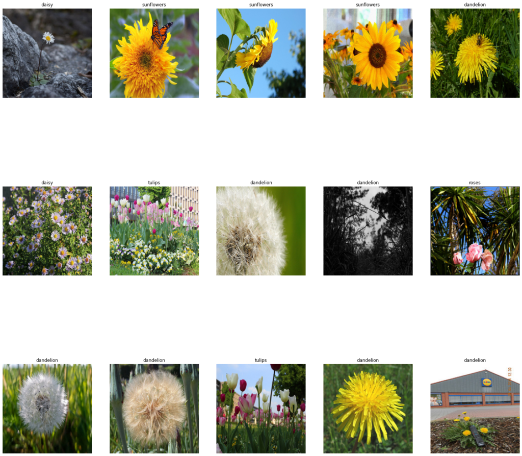

Now we will generate some Augmented images using the trained generator. Notice how images are rotated, zoomed, etc.

# Display Augmented Images
display_images(train_data_generator)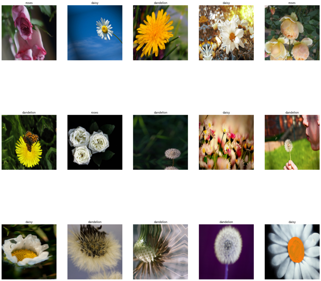

Create the Model

Since we’re using Tensorflow 2 (TF2) and in TF2 the most popular way to go about creating neural networks is by using the Keras API. Previously Keras used to be a separate framework (it still is) but not so long ago because of Keras’ popularity in the community it was included in TensorFlow as the default high-level API. This abstraction allows developers to use TensorFlow’s low-level functionality with high-level Keras code. 

This way you can design powerful neural networks in just a few lines of code. E.g. take a look at how we have created effective Convolutional Networks.

# First Reset the generators, since we used the first batch to display the images.
vald_data_generator.reset()
train_data_generator.reset()

# Here we are creating Sequential model also defing its layers
model = Sequential([
      Conv2D(16, 3, padding='same', activation='relu', input_shape=(IMG_HEIGHT, IMG_WIDTH ,3)),
      MaxPooling2D(),
      Dropout(0.10),

      Conv2D(32, 3, padding='same', activation='relu'),
      MaxPooling2D(),

      Conv2D(64, 3, padding='same', activation='relu'),
      MaxPooling2D(),

      Conv2D(128, 3, padding='same', activation='relu'),
      MaxPooling2D(),

      Conv2D(256, 3, padding='same', activation='relu'),
      MaxPooling2D(),
    
      GlobalAveragePooling2D(),
      Dense(1024, activation='relu'),
      Dropout(0.10),
      Dense(len(classes), activation ='softmax')
  ])

A typical neural network has a bunch of layers, in a Convolutional network, you’ll see convolutional layers. These layers are created with the Conv2d function. Take a look at the first layer:

      Conv2D(16, 3, padding=’same’, activation=’relu’, input_shape =(IMG_HEIGHT, IMG_WIDTH ,3))

The number `16` refers to the number of filters in that layer, normally we increase the number of filters as you add more layers. You should notice that I double the number of filters in each subsequent convolutional layer i.e. 16, 32, 64 …, this is common practice. In the first layer, you also specify a fixed input shape that the model will accept, which we have already set as 200x200

Another thing you’ll see is that typically a convolutional layer is followed by a pooling layer. So the Conv layer outputs a number of feature maps and the pooling layer reduces the spatial size (width and height) of these feature maps which effectively reduces the number of parameters in the network thus reducing computation.

So you’ll commonly have a convolutional layer followed by a pooling layer, this is normally repeated several times, at each stage the size is reduced and the no of filters is increased. We are using a MaxPooling layer there are other pooling types too e.g. AveragePooling.

The Dropout layer randomly drops x% percentage of parameters from the network, this allows the network to learn robust features. In the network above I’m using dropout twice and so in those stages I’m dropping 10% of the parameters. The whole purpose of the Dropout layer is to reduce overfitting.

Now before we add the final layer we need to flatten the output in a single-dimensional vector, this can be done by the flatten layer but a better method is using the  GlobalAveragePooling2D Layer, which flattens the output while reducing the parameters.

Finally, before our last layer, we also use a Dense layer (A fully connected layer) with 1024 units. The final layer contains the number of units equal to the number of classes. The activation function here is softmax as I want the network to produce class probabilities at the end.

Compile the model

Before we can start training the network we need to compile it, this is the step where we define our loss function, optimizer, and metrics.

For this example, we are using the ADAM optimizer and a categorical cross-entropy loss function as we’re dealing with a multi-class classification problem. The only metric we care about right now is the accuracy of the model.

# Compile the model
model.compile(optimizer=Adam(learning_rate=0.001), loss='categorical_crossentropy', metrics=['accuracy'])

Model summary

By using the built-in method called summary() we can see the whole architecture of the model that we just created. You can see the total parameter count and the number of params in each layer.

model.summary()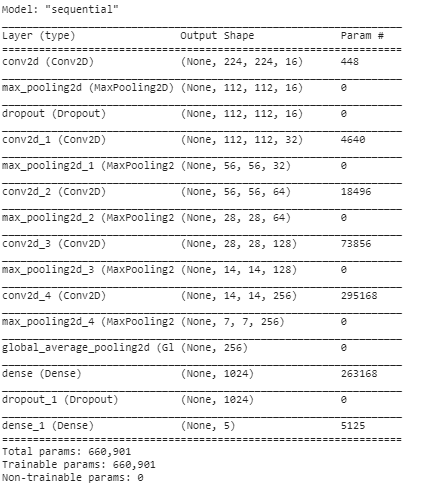

Notice how the number of params is `0` in all layers except the Conv and Dense layers, this is because these are the only two types of layers here which are actually involved in learning.

Training the Model:

You can start training the model using the model.fit() method but first, specify the number of epochs, and the steps per epoch. 

Epoch: A single epoch means 1 pass of the whole data meaning an epoch is considered done when the model goes over all the images in the training data and uses it for gradient calculation and optimizations. So this number decides how many times the model will go over your whole data.

Steps per epoch: A single step means the model goes over a single batch of the data, so steps per epoch tells, after how many steps should an epoch be considered done. This should be set to `dataset_size / batch_size` which is the number of steps required to go over the whole data once.

Let’s train our model for `60` epochs.

# Define the epoch number 
epochs = 60

# Start Training
history = model.fit( train_data_generator,  steps_per_epoch= train_data_generator.samples // batch_size, epochs=epochs, validation_data= vald_data_generator,
    validation_steps = vald_data_generator.samples // batch_size )

# Use model.fit_generator() if using TF version < 2.2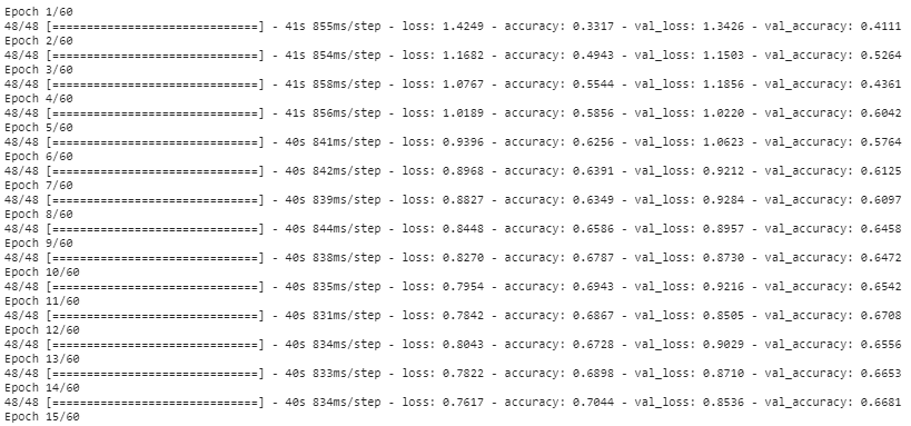

…………………………………..
…………………………………..

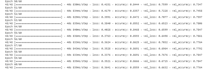
You can see in the last epoch that our validation loss is low and accuracy is high so our model has successfully converged, we can further verify this by plotting the loss and accuracy graphs.

After you’re done training it’s a good practice to plot accuracy and loss graphs.

# Plot the accuracy and loss curves for both training and validation

acc = history.history['accuracy']
val_acc = history.history['val_accuracy']
loss = history.history['loss']
val_loss = history.history['val_loss']

epochs = range(len(acc))

plt.plot(epochs, acc, 'b', label='Training acc')
plt.plot(epochs, val_acc, 'r', label='Validation acc')
plt.title('Training accuracy')
plt.legend()

plt.figure()

plt.plot(epochs, loss, 'b', label='Training loss')
plt.plot(epochs, val_loss, 'r', label='Validation loss')
plt.title('Training loss')
plt.legend()

plt.show()

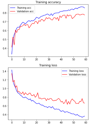
The model has slightly overfitted at the end but that is okay considering the number of images we used and our model’s capacity.

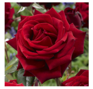
You can test out the trained model on a single test image using this code. Make sure to carry out the same preprocessing steps you used before training for e.g. since we trained on normalized images in range 0-1, we will need to divide any new image with 255 before passing it to the model for prediction.

# Read the rose image
img = cv2.imread('rose.jpg')

# Resize the image to the size you trained on.
imgr= cv2.resize(img,(224,224))

# Convert image BGR TO RGB, since OpenCV works with BGR and tensorflow in RGB.
imgrgb = cv2.cvtColor(imgr, cv2.COLOR_BGR2RGB)

# Normalize the image to be in range 0-1 and then convert to a float array.
final_format = np.array([imgrgb]).astype('float64') / 255.0

# Perform the prediction
pred = model.predict(final_format)

# Get the index of top prediction
index = np.argmax(pred[0])

# Get the max probablity for that prediction
prob = np.max(pred[0])

# Get the name of the predicted class using the index
label = classes[index]

# Display the image and print the predicted class name with its confidence.
print("Predicted Flowers is : {} {:.2f}%".format(label, prob*100))
plt.imshow(img[:,:,::-1]);plt.axis("off");

Predicted Flowers is : roses, 85.61%

Notice that we are converting our model from BGR to RGB color format. This is because TensorFlow has trained the model using images in RGB format whereas OpenCV reads images in BGR format, so we have to reverse channels before we can perform prediction.

Finally, when you’re satisfied with the model you save it in .h5 format using the model.save function.

# Saving your model to disk allows you to use it later
model.save('flowers.h5')

# Later on you can load your model this way
#model = load_model('Model/flowers.h5')

Part 2: Converting Our Classifier to ONNX format

Now that we have trained our model, it’s time to convert it to ONNX format.

What is ONNX?

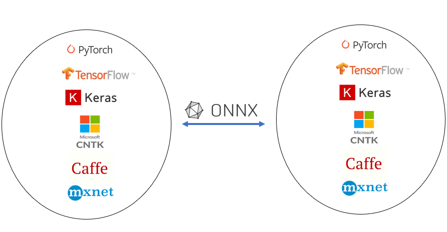
ONNX stands for Open neural network exchange. ONNX is an industry-standard format for changing model frameworks, this means you can train a model in PyTorch or any other common frameworks and then convert to onnx and then convert back to TensorFlow or any other framework. 

So ONNX allows developers to move models between different frameworks such as CNTK, Caffe2, Tensorflow, PyTorch, etc.

So why are we converting to ONNX?

Remember our goal is to use the above custom trained model in the DNN module but the issue is the DNN module does not support using the .h5 Keras model directly. So we have to convert our .h5 model to a .onnx model after doing this we will be able to take the onnx model and plug it into the DNN module.

Note: Even if you saved the model in saved_model format then you still can’t use it directly 

You need to use keras2onnx module to perform the conversion so you should go ahead and install the keras2onnx module.

pip install keras2onnx

You also need to install onnx so that you can save .onnx models to disk.

pip install onnx

After installing keras2onnx, you can use its convert_keras function to convert the model, we will also serialize the model to disk using keras2onnx.save_model  so we can use it later.

# Import keras2onnx and onnx
import onnx
import keras2onnx

# Load the keras model
model = load_model('flowers.h5')

# Convert it into onnx
onnx_model = keras2onnx.convert_keras(model, model.name)

# Save the model as flower.onnx
onnx.save_model(onnx_model, 'flowers_model.onnx')

tf executing eager_mode: True
tf.keras model eager_mode: False
The ONNX operator number change on the optimization: 57 -> 25

Now we’re ready to use this model in the DNN module. Check how your ~7.5 MB .h5 model now has reduced to ~2.5 MB .onnx model, a 3x reduction in size. Make sure to check out  keras2onnx repo for more details.

Note: You can even use this model with just ONNX using onnxruntime module which itself is pretty powerful considering the support of multiple hardware accelerations.

Using the ONNX model in the OpenCV DNN module:

Now we will take this ONNX model and use it directly in our DNN module.

Let’s use this as a test image.

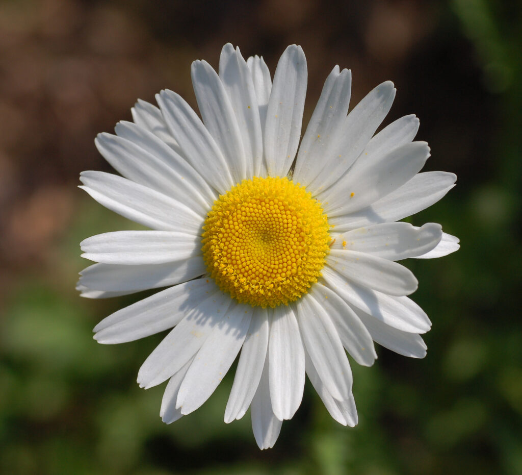
Here’s the code to test the ONNX model on the image.

# Make sure your version is 4.0.0
import cv2
import numpy as np

# Define class names and sort them alphabatically as this is how tf.keras remembers them 
label_names = ['daisy','dandelion','roses','sunflowers','tulips']
label_names.sort()

# Read the ONNX model
net = cv2.dnn.readNetFromONNX('flowers_model.onnx')

# Read the image
img_original = cv2.imread('daisy.jpg')

img = img_original.copy()
# Resize Image
img = cv2.resize(img_original,(224,224))

# Convert BGR TO RGB
img = cv2.cvtColor(img, cv2.COLOR_BGR2RGB)

# Normalize the image and format it
img = np.array([img]).astype('float64') / 255.0

# Input Image to the network
net.setInput(img)

# Perform a Forward pass
Out = net.forward()

# Get the top predicted index
index = np.argmax(Out[0])

# Get the probability of the class.
prob = np.max(Out[0])

# Get the class name by putting index number
label =  label_names[index]
text = "Predicted: {} {:.2f}%".format(label, prob)

# Write predicted flower on image
cv2.putText(img_original, text, (5, 4*26),  cv2.FONT_HERSHEY_COMPLEX, 4, (100, 20, 255), 6)
 
# Display image
plt.figure(figsize=(10,10))
plt.imshow(img_original[:,:,::-1]);
plt.axis("off");

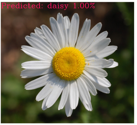
Here’s the result of a few images which I took from google, I’m using my custom function classify_flower() to classify these images. You can find this function’s code inside the downloaded Notebook.

# Initialize the Network
init_classify()

# Classify on image
img = cv2.imread("Images/sunflower.jpg");
classify_flower(img,size=8);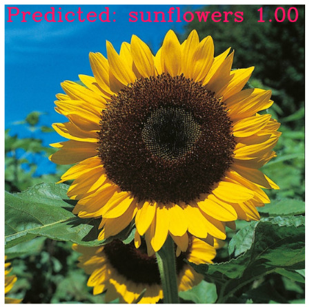

img = cv2.imread("Images/tulip.jpg");
classify_flower(img,size=2);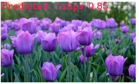

img = cv2.imread("Images/dandelion.jpg");
classify_flower(img,size=3);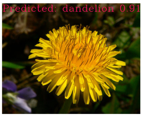

img = cv2.imread("Images/daisy0.jpg");
classify_flower(img,size=2);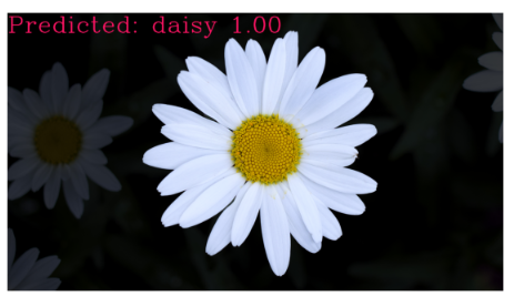

If you want to learn about doing image classification using the DNN module in detail then make to read the previous post,  Deep learning with OpenCV DNN module. Where I have explained each step in detail.

Summary:

In today’s post we first learned how to train an image classifier with tf.keras, after that we learned how to convert our trained .h5 model to .onnx model.

Finally, we learned to use this onnx model using OpenCV’s DNN module.

Although the model we converted today was quite basic but this same pipeline can be used for converting complex models too.

A word of Caution: I personally have faced some issues while converting some types of models so the whole process is not foolproof yet but it’s still pretty good. Make sure to look at keras2onnx repo and this excellent repo of ONNX conversion tutorials.

You can reach out to me personally for a 1 on 1 consultation session in AI/computer vision regarding your project. Our talented team of vision engineers will help you every step of the way. Get on a call with me directly here.

You can reach out to me personally for a 1 on 1 consultation session in AI/computer vision regarding your project. Our talented team of vision engineers will help you every step of the way. Get on a call with me directly here.