Computer Vision Crash Course with OpenCV & Python
If you’re looking for a single stand-alone Tutorial that will give you a good overall taste of the exciting field of Computer Vision using OpenCV then this is it. This Tutorial will serve as a Crash Course to learn the basics of OpenCV Library.
What is OpenCV:
OpenCV (Open Source Computer Vision ) is the biggest library for Computer Vision which contains more than 2500 optimized algorithms that can be used to do face detection, action recognition, image stitching, extracting 3d models, generating point clouds, augmented reality and a lot more.
So if you’re planning to perform Computer Vision weather on a deep learning project or on a Raspberry pie or you want to make a career in it then at some point you will definitely cross paths with this library. So it’s better that you get started with it today.
About this Crash Course Course:
Since I’m a member of the Official OpenCV.org Course team and this blog Bleed AI is all about making you master Computer Vision, so I feel I’m in a very good position to teach you about this library and that too in a single post.
Of Course, we won’t be able to cover a whole lot as I said it contains over 2500 algorithms, still, after going through this course you will be able to get a grip on fundamentals and built some interesting things.
Prerequisite: To follow along with this course it’s important that you are familiar with Python language & you have python installed in your system.
Make sure to download the Source code below to try out the code.
[optin-monster slug=”hdos5xtdkhuhlaq3bz0j”]
Let’s get Started
Crash Course Outline:
Here’s the outline for this course.
- OpenCV Installation
- Reading & Displaying an Image
- Accessing & Modifying Image Pixels & ROI
- Resizing the Image
- Drawing Shapes on Images
- Cropping the Image.
- Image Smoothing/Blurring
- Thresholding
- Edge detection
- Morphological Operations
- Working with Videos
- Machine Learning-based Face Detector
- Deep Learning with OpenCV
Installing OpenCV-python:
The easiest way to install OpenCV is by using a package manager like e.g. with pip.
So you can just Open Up the command prompt and run the following command:
pip install opencv-contrib-python
By doing the above, you will install opencv along with its contrib package which contains some extra algorithms. If you don’t need the extra algorithms then you can also run the following command:
pip install opencv-python
Make sure to install Only one of the above packages, not both. There are also some headless versions of OpenCV which do not contain any GUI functions, you can look those here.
The other Method to install OpenCV is installing it from the source. Now installing from the source has its perks but it’s much harder and I recommend only people who have prior experience with OpenCV attempting this. You can look at my tutorial of installing from the source here.
Note: Before you can install OpenCV, you must have numpy library installed on your system. You can install numpy by doing:
pip install numpy
After Installing OpenCV you should check your installation by opening up the command prompt or anaconda prompt, launching python interpreter by typing `python` and then importing OpenCV by doing: import cv2

Reading & Displaying an Image:
After installing OpenCV we will see how we can read & display an image in OpenCV. You can start by running the following cell in the jupyter notebook you downloaded from the source code section.
In OpenCV you can read an image by using the cv2.imread() function.
image = cv2.imread(filename, [flag])
Note: The Square brackets i.e. [ ] are used to denote optional parameters
Params:
- filename: Name of the image or path to the image.
- flag: There are numerous flags but three most important ones are these:
0,1,-1
If you pass in 1 the image is read in Color, if 0 is passed the image is read in Grayscale (Black & white) and if -1 is used to read transparent images which we will learn in the next chapter, If no parameter is passed the image will be read in Color.
# This is how you import the Opencv Library
import cv2

# We will also import numpy library as np
Import numpy as np

# Read the Image
img = cv2.imread('Media/M1/two.png',0)

# Print the image
print(img)
Line 1-5: Importing Opencv and numpy library.
Line 8: We are reading our image in grayscale, this function will read the image in a numpy array format.
Line 11: We are printing our image.
Output:
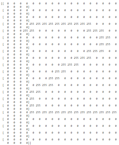
Now just by looking at the above output, you can get a lot of information about the image we used.
Take a guess on what’s written in the image.
Go ahead …I’ll wait.
If you guessed the number 2 then congrats you’re right. In fact, there is a lot more information that you can extract from the above output. For e.g, I can tell that the size of the image is (21x22). I can also say that number 2 is written in white on a black image and is written in the middle of the image.
How was I able to get all that…especially considering I’m no Sherlock?
The size of the image can easily be extracted by counting the number of rows & columns. And since we are working with a single channel grayscale image, the values in the image represent the intensity of the image, meaning 0 represents black and 255 white color, and all the numbers between 0 and 255 are different shades of gray.
You can look at the colormap below of a Grayscale image to understand it better.

Beside’s counting the rows and columns, you can just use the `shape` function on a numpy array to find its shape
Img.shapeOutput:
(21, 22)
The values returned are in rows, columns or you can call it height, width, or x,y. If we were dealing with a color image then img.shape would have returned height, width, channels.
Now it’s not ideal to print images, especially when they are 100s of pixels in width and height, so let’s see how we can show images with OpenCV.
To display an Image there are generally 3 steps. There are generally 3 steps involved in displaying an image properly.
Step 1: Use cv2.imshow() to show images.
Params:
- Window_Name: Any custom name you assign to your window
- img: Your image either be in uint8 datatype or float datatype having range
0-1.
Step 2: Also with cv2.imshow() you will have to use the cv2.waitKey() function. This function is a keyboard binding function. Its argument is the time in milliseconds. The function waits for specified milliseconds. If you press any key in that time frame, the program continues. If 0 is passed, it waits indefinitely for a keystroke. This function returns the ASCII value of the keyboard key pressed, for e.g. if you press ESC key then it will return 27 which is the ASCII value for the ESC key. For now, we won’t be using this returned value.
Note: The default delay is 0 which means wait forever until the user presses a key.
Step 3: The last step is to destroy the window we created so the program can end, now this is not required to view the image but if you don’t destroy the window then you can’t proceed to end the program and it can crash, so to destroy the windows you will do:
This will destroy all present image windows, there is also a function to destroy a specific window.
Now let’s see the full code in action.
# Read the image
img = cv2.imread('Media/two.png',0)

# Resize the image to 1000% in size since its too small
img = cv2.resize(img, (0,0), fx=10, fy=10)

# Display the  image
cv2.imshow("Image",img)

# Wait for the user to press any key
cv2.waitKey(0)

# Destroy all windows
cv2.destroyAllWindows()
Line 5: I’m resizing the image by 1000% or by 10 times in both x and y direction using the function cv2.resize() since the original size of the image is too small. I will later discuss this function.
Line 8-14: Showing the image and waiting for a keypress. Destroying the image when there is a keypress.
Output:

Accessing & Modifying Image Pixels and ROI:
For this example, I will be reading this image which is from one of my favorite Anime series.

You can access individual pixels of the image and modify them. Now before we get into that lets understand how an image is represented in OpenCV. We already know it’s a numpy array. But besides that you can find out other properties of the image.
img = cv2.imread('Media/naruto.jpg',1)

print('The data type of the Image is: {}'.format(img.dtype))
print('The dimensions of the Image is: {}'.format(img.ndim))
Output:
The data type of the Image is: uint8
The dimensions of the Image is: 3
So the datatype of images you read with OpenCV is uint8 and if its a color image then it’s a 3-dimensional image.
Let’s talk about these dimensions. First 2 are the width and the height and the 3rd are the image channels. Now these are B (blue), G (green), & R (red) channels. In OpenCV due to historical reasons, colored images are stored in BGR instead of the common RGB format.

You can access any individual pixel value bypassing its x,y location in the image.
print(img [300, 300])
Output:
[143 161 168]
The tuple output above means that at location (300,300) the value for the blue channel is 143, the green channel is 161 and the red channel is 168.
Just like we can read individual image pixels, we can modify them too.
img[300,300] = 0
I’ve just made the pixel at location (300,300) black. Because I’ve only modified a single pixel the change is really hard to see. So now we will modify an ROI (Region of Interest) of the image so that we can see our changes.
Modifying a whole ROI is pretty similar to modifying a pixel, you just need to select a range instead of a single value.
# Make a copy of the original Image
Img_copy = img.copy()

# Modify the ROI
Img_copy[100:150,80:120]  =  0

# Display image
cv2.imshow("Fixed Resizing",Img_copy)
cv2.waitKey(0)
cv2.destroyAllWindows()
Line 1-2: We are making a copy of the image so we don’t end up modifying the original.
Line 4-5: We are setting all pixels in x range 100-150 and in y range 80-120 equal to 0 (meaning black). Now, this should give us a black box in the image.
Line 8-10 : Showing the image and waiting for a keypress. Destroying the image when there is a keypress.
Output:

Resizing an Image:
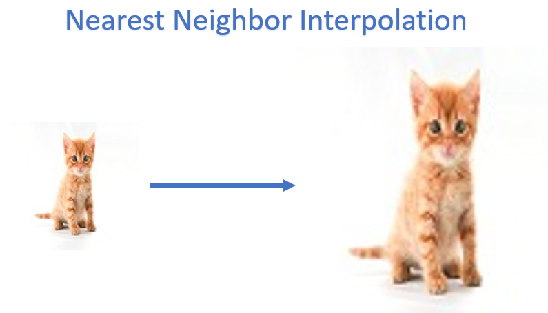
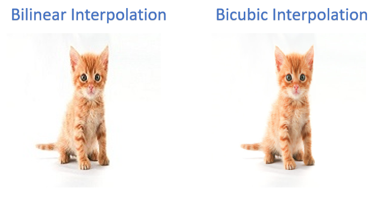
You can use cv2.resize() function to resize an image. You have 2 ways of resizing the image, either by passing in the new width & height values or by passing in percentages of those values using fx and fy params. We have already seen how we used the second method to resize the image to 10x its size so now I’m going to show you the first method.
# Read image in color
img = cv2.imread('Media/narutosage.jpg',1)
# Resizing image to a fix 300x300 size
resized = cv2.resize(img, (300,300))
# Display image
cv2.imshow("Fixed Resizing", resized);
cv2.waitKey(0)
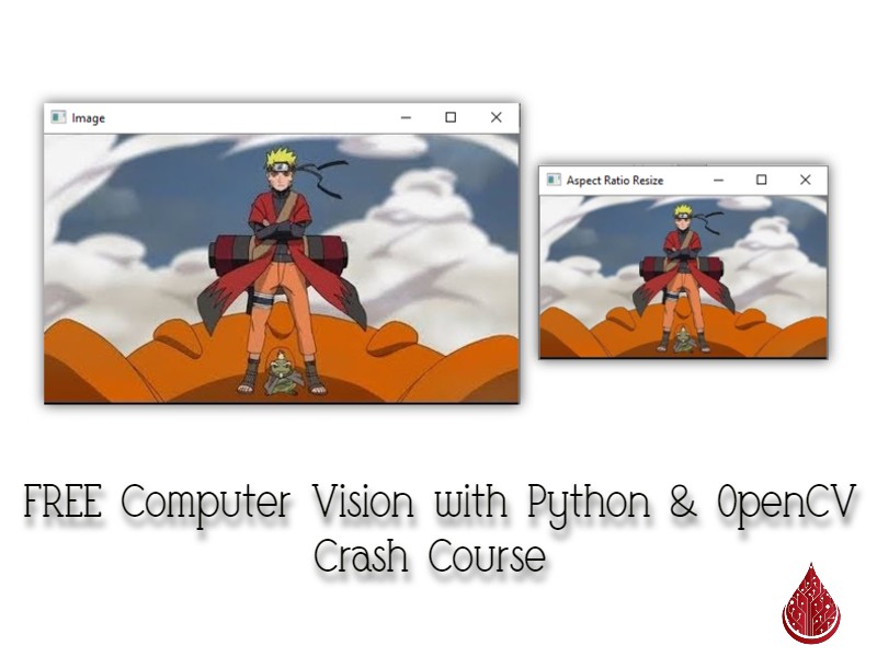
cv2.destroyAllWindows()You can see below both the original and the resized version of the image.
Result:

An obvious problem with the above approach you can see is that it’s not maintaining the aspect ratio of the image which is why the image looks distorted to you. A better approach would be to resize a single dimension at a time and shrink or expand the other dimension accordingly.
Resizing While Keeping the Aspect Ratio Constant:
So let’s resize the image while keeping the aspect ratio constant. This time we are going to resize the width to 300 and modify the height respectively.
# Read image in color
img = cv2.imread('Media/narutosage.jpg',1)

# Get the width and height of image
height, width =  img.shape[:-1]

# Compute ratio for the new height taking into account the 300 px width of image
r = 300.0 / width

# Get the new height
new_height = int(height * r)

# Resize the image with 300 width and the new height.
resized = cv2.resize(img, (300, new_height))

# Display Resized Image
cv2.imshow("Aspect Ratio Resize", resized)
cv2.waitKey(0)
cv2.destroyAllWindows()
Line 4-5: We are extracting the shape of the image, [:-1] indicates that I don’t want channels returned, just height and width. This ensures your code works for both color and grayscale images.
Line 7-11: We are calculating the ratio of the new width to the old width and then multiplying this ratio value with the height for getting the new value of the height. The logic behind is this, if we resized a 600 px width image to 300 px width then we would get a ratio of 0.5 and if the height was 200 px then by multiplying 0.5 with the height, we would get a new value of 100 px, by using these new values we won’t get any distortions.
Result:

Geometric Transformations:
You can apply different kinds of transformations to the image, now there are some complex transformations but for this post, I will only be discussing translation & rotation. Both of these are types of Affine transformations. So we will be using a function called warpAffine() to transform them.
transformed_ image = cv2.warpAffine(src, M, dsize[, dst[, flags[, borderMode[, borderValue]]]])
Params:
- src: input image.
- M: 2×3 transformation matrix.
- dsize: size of the output image.
- flags: combination of interpolation methods.
- borderMode: pixel extrapolation method (see BorderTypes) by default its constant border.
- borderValue: value used in case of a constant border; by default, it is
0, which means replaced values will be black.
Now you pass in a 2×3 Matrix into the warpaffine function which does the required transformation, the first two 2 columns of the matrix control, rotation, scale and shear, and the last column encodes translation (shift) of image.

Again, we will only focus on translation and rotation in this post.
Translation:
Translation is the shifting of an object’s location, meaning the movement of image in x, y-direction. Suppose you want the image to move tx amount of pixels in the x-direction and ty amount of pixels in y-direction then you will construct below transformation matrix accordingly and pass it into the warpAffine function.
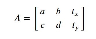
So now you just need to change the tx and ty values here for translation in x and y direction.
# Read Image
img = cv2.imread('media/naruto.jpg')

rows, cols, channels = img.shape

# Construct the translation matrix
M = np.float32([
    [1,0, 120],
    [0,1, -40]
])

# Apply the warpAffine function
translated = cv2.warpAffine(img, M, (cols,rows))

# Display image
cv2.imshow("Translated Image",translated);
cv2.waitKey(0)
cv2.destroyAllWindows()
Line 6-10: We’re constructing the translation matrix so we move 120 px in x-direction and 40 px in the negative y-direction.
Output:

Rotation
Similarly, we can also rotate an image, by passing a matrix into the warpaffine function. Now instead of designing a matrix for rotation, I’m going to use a built-in function called cv2.getRotationMatrix2D() which will return a rotation matrix according to our specifications.
M = cv2.getRotationMatrix2D( center, angle, scale )
Params:
- center: This is the center of the rotation in the source image.
- Angle: The Rotation angle in degrees. Positive values mean counter-clockwise rotation (the coordinate origin is assumed to be the – top-left corner).
- Scale: scaling factor.
# Set angle to 45 degrees.
angle = 45

# Rotate image from center of image with an angle of 45 degrees at the same scale.
rotation_matrix = cv2.getRotationMatrix2D((cols/2,rows/2), angle, 1)

# Apply the transformation
rotated = cv2.warpAffine(img, rotation_matrix, (cols,rows))

# Display image
cv2.imshow("Rotated Image",rotated);
cv2.waitKey(0)
cv2.destroyAllWindows()
Output:

Note: If you don’t like the black pixels that appear after translation or rotation then you can use a different border filling method, look at the available borderModes here.
Drawing on Image:
Let’s take a look at some drawing operations in OpenCV. So now we will learn how to draw a line, a circle, and a rectangle on an image. We will also learn to put text on the image. Since each drawing function will modify the image so we will be working on copies of the original image. We can easily make a copy of image by doing: img.copy()
Most of the drawing functions have below parameters in common.
- img : Your Input Image
- color : Color of the shape for a BGR image, pass it as a tuple i.e. (255,0,0), for Grayscale image just pass a single scalar value from
0-255. - thickness : Thickness of the line or circle etc. If
-1is passed for closed figures like circles, it will fill the shape. default thickness =1 - lineType : Type of line, popular choice is
cv2.LINE_AA.
Drawing a Line:
We can draw a line in OpenCV by using the function cv2.line(). We know from basic geometry you can draw a line, you just need 2 points. So you’ll pass in coordinates of 2 points in this function.
cv2.line(img, pt1, pt2, color, [thickness])
Params:
- pt1: First point of the line, this is a tuple of (x1,y1) point.
- pt2: Second point of the line, this is a tuple of (x2,y2) point.
# Make a copy of the original image
copy = img.copy()

# Draw a line on the image with these parameters.
cv2.line(copy, (400,250),(300,30), (255,255,0), 5)

# Display image
cv2.imshow("Draw Line", copy);
cv2.waitKey(0)
cv2.destroyAllWindows()
Output:

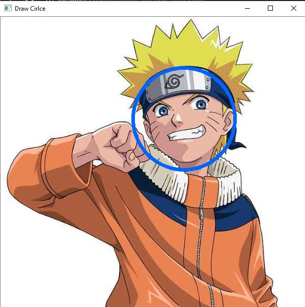
Drawing a Circle
We can draw a Circle in OpenCV by using the function `cv2.Circle()`. For drawing a circle we just need a center point and a radius.
cv2.circle(img, Center, radius, color, [thickness])
Params:
- center: Center of the circle.
- radius: Radius of the circle.
# Make a copy of the original image
copy = img.copy()

# Draw a Circle on naruto’s face with a radius of a 100.
cv2.circle(copy, (360,200), 100, (255,100,0), 5)

# Display image
cv2.imshow("Draw Circle", copy);
cv2.waitKey(0)
cv2.destroyAllWindows()
Output:
Drawing a Rectangle
We can also draw a rectangle in OpenCV by using the function cv2.rectangle(). You just have to pass two corners of a rectangle to draw it. It’s similar to the cv2.line function.
cv2.rectangle(img, pt1, pt2, color, [thickness])
Params:
- pt1: Top left corner of the rectangle.
- pt2: bottom right corner of the rectangle.
# Make a copy of the original image
copy = img.copy()

# Draw Rectangle around Naruto's face.
cv2.rectangle(copy, (250,100), (450,300), (0,255,0),3)

# Display image
cv2.imshow("Draw Rectangle", copy);
cv2.waitKey(0)
cv2.destroyAllWindows()
Output:

Putting Text:
Finally, we can also write Text by using the function cv2.putText(). Writing Text on images is an essential tool, you will be able to see real-time stats on image instead of just printing. This is really handy when you’re working with videos.
cv2.putText(img, text, origin, fontFace, fontScale, color, [thickness])
Params:
- text: Text string to be drawn.
- origin: Top-left corner of the text (x,y) origin position.
- fontFace: Font type, we will use cv2.FONT_HERSHEY_SIMPLEX.
- fontScale: Font scale, how large your text will be.
# Make a copy of the original image
copy = img.copy()

# Write ‘Bleed AI’ on the image
img= cv2.putText(img,'Bleed-AI',(250,470),cv2.FONT_HERSHEY_SIMPLEX, 1.7, (255,255,0), 4)

# Display image
cv2.imshow("Write Text",img);
cv2.waitKey(0)
cv2.destroyAllWindows()
Output:

Cropping an Image:
We can also crop or slice an image, meaning we can extract any specific area of the image using its coordinates, the only condition is that it must be a rectangular area. You can segment irregular parts of images but the image is always stored as a rectangular object in the computer, this should not be a surprise since we already know that images are matrices. Now let’s say we wanted to crop naruto’s face then we would need four values namely X1 (lower bound on the x-axis), X2 (Upper bound on y-axis), Y1 (lower bound on the y-axis) and Y2 (Upper bound on the y-axis).
After getting these values, you will pass them in like below.
`face_roi = img [Start X : End X, Start Y: End Y]`
Lets see the full script
# Grab the Face ROI
face_roi  = img[100:270,300:450]

# Display image
cv2.imshow("Image",face_roi);
cv2.waitKey(0)
cv2.destroyAllWindows()
Line 2: We are passing in the coordinates to crop naruto’s face, you can get these coordinates by several methods, some are of them are: by trial and error, by hovering the mouse over the image when using `matplotlib notebook` magic command, or by hovering over the image when you have installed OpenCV with QT support or by making a mouse click function that splits x,y coordinates.
Result:

Note: If you’re gonna modify the cropped ROI, then it’s better to make a copy of it, otherwise modifying the cropped version would also affect the original.
You can make a copy like this:
face_roi = img[100:270,300:450].copy()
Image Smoothing/Blurring:
Smoothing or blurring an Image in OpenCV is really easy. If you’re thinking about why we would need to blur an image then understand that It’s very common to blur/smooth an image in vision applications, this reduces noise in the image. The noise can be present due to various factors like maybe the sensor by which you took the picture was corrupted or it malfunctioned, or environmental factors like the lightning was poor, etc. Now there are different types of blurring to deal with different types of noises and I have discussed each method in detail and even done a comparison between them inside our Computer Vision Course but for now, we will briefly look at just one method, the Gaussian Blurring method. This is the most common image smoothing technique used. It gets rid of Gaussian Noise. In simple words, this will work most of the time.
Smoothed_image = cv2.GaussianBlur(source-image, ksize, sigmaX)
Params:
- source-image: Our input image
- ksize: Gaussian kernel size. kernel width and height can differ but they both must be positive and odd.
- sigmaX: Gaussian kernel standard deviation in X direction.
Again to keep this short, I won’t be getting into the math nor the parameter details for how this function works, although it’s really interesting. One thing you need to learn is that by controlling the kernel size you control the level of smoothing done. There is also a SigmaX and a SigmaY parameter that you can control.
# Blur the image
blurred = cv2.GaussianBlur(img,(9,9), 50)

# Display blurred image
cv2.imshow("Blur",blurred);
cv2.waitKey(0)
cv2.destroyAllWindows()
Output:

Thresholding an Image:
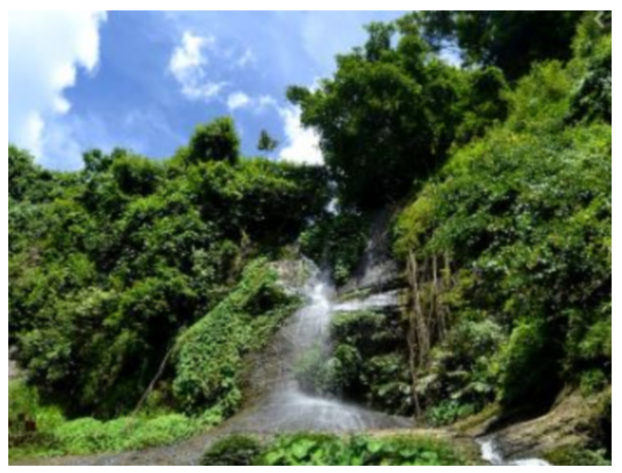
For this section, we will be using this image.

There are times when we need a binary black & white mask of the image, where our target object is in white and the background black or vice versa. The easiest way to get a mask of our image is to threshold our image. There are different types of thresholding methods, I’ve introduced most of them in our Computer Vision course but for now, we are going to discuss the most basic and most used one. So what thresholding does is that it checks each pixel in the image against a threshold value and If the pixel value is smaller than the threshold value, it is set to 0, otherwise, it is set to the maximum value, (this maximum value is usually 255 so white color).
ret, thresholded_image = cv2.threshold(source_image, thresh, max_value, type)
Params:
- Source_image: This is your input image.
- thresh: Threshold value. (If you use THRESH_BINARY then all values above this are set to max_value.)
- max_value: Maximum value, normally this is set to be
255. - type: Thresholding type. The most common types are THRESH_BINARY & THRESH_BINARY_INV
- ret: Boolean variable which tells us if thresholding was successful or not.
Now before you can threshold an image you need to convert the image into grayscale, now you could have loaded the image in grayscale but since we have a color image already we can convert to grayscale using cv2.cvtColor function. This function can be used to convert one color to different color formats for this post we are only concerned with the grayscale conversion.
# Read the image
img = cv2.imread('media/shapes.jpg')

# Convert the color image to grayscale
gray_image = cv2.cvtColor(img, cv2.COLOR_BGR2GRAY)

# Display the grayscale image.
cv2.imshow("Grayscale Image", gray_image);
cv2.waitKey(0)
cv2.destroyAllWindows()
Output:

Now that we have a grayscale image, we can apply our threshold.
# Apply the threshold
_ , thresholded_image = cv2.threshold(gray_image, 220, 255, cv2.THRESH_BINARY)

# Display Thresholded image
cv2.imshow("Thresholded Image",thresholded_image);
cv2.waitKey(0)
cv2.destroyAllWindows()
Line 2: We are applying a threshold such that all pixels having an intensity above 220 are converted to 255 and all pixels below 220 become 0.
Output:

Now Let’s see the result of the inverted threshold, which just reverses the results above. For this you just need to pass in cv2.THRESH_BINARY_INV instead of cv2.THRESH_BINARY.
# Apply the threshold
_ , thresholded_image = cv2.threshold(gray_image, 220, 255, cv2.THRESH_BINARY_INV)

# Display Threshold image
cv2.imshow("Thresholded Image", thresholded_image);
cv2.waitKey(0)
cv2.destroyAllWindows()
Output:

Edge Detection:
Now we will take a look at edge detection, why edge detection? Well edges encode the structure of the images and it encodes most of the information in the images so for this reason edge detection is an integral part of many Vision applications.
In OpenCV there are edge detectors such as Sobel filters and laplacian filters but the most effective is the Canny Edge detector. In our Computer Vision Course I go into detail of exactly how this detector works but for now let’s take a look at its implementation in OpenCV.
edges = cv2.Canny( image, threshold1, threshold2)
Params:
- image: This is our input image.
- edges: output edge map; single channels 8-bit image, which has the same size as image .
- threshold1: First threshold for the hysteresis procedure.
- threshold2: Second threshold for the hysteresis procedure.
# Detect Edges in image
edges = cv2.Canny(img, 30, 150)

# Display images
cv2.imshow("Edge Detection", edges);
cv2.waitKey(0)
cv2.destroyAllWindows()
Line 1-2: I’m detecting edges with lower and upper hysteresis values being 30 and 150. I can’t explain how these values work without going into the theory so, for now, understand that for any image you need to tune these 2 threshold values to get the correct results.
Output:

Contour Detection:
Contour detection is one of my most favorite topics because with just contour detection you can do a lot and I’ve built a number of cool applications using contours.
Contours can be defined simply as a curve joining all the continuous points (along the boundary), having the same color or intensity. In simple terms think of contours as white blobs on black background for e.g. in the output of threshold function or the edge detection function, each shape can be considered as an individual contour. So you can segment each shape, localize them or even recognize them.
The contours are a useful tool for shape analysis, object detection, and recognition, take a look at this detection and recognition application I’ve built using contour detection.
You can use this function to detect contours.
contours, hierarchy = cv2.findContours(image, mode, method[, offset])
Params:
- image Source: This is your input image in binary format, this is either a black & white image obtained from a thresholding or a similar function or the output of a canny edge detector.
- mode: Contour retrieval mode, for example cv2.RETR_EXTERNAL mode lets you extract only external contours meaning if there is a contour inside a contour then that child contour will be ignored. You can see other RetrievalModes here
- method: Contour approximation method, for most cases cv2.CHAIN_APPROX_NONE works just fine.
After you detect contours you can draw them on the image by using this function.
cv2.drawContours( image, contours, contourIdx, color, [thickness] )
Params:
- image: original input image.
- contours: This is a list of contours, each contour is stored as a vector.
- contourIdx: Parameter indicating which contour to draw. If it is
-1then all the contours are drawn. - color: Color of the contours.
# Make a copy of the original image so it won’t be corrupted during drawing
image_copy   = img.copy()

# Alternatively you can also pass in the edges output to the contours function.
# Threshold image, Remember the target object is white and background black.
gray_image = cv2.cvtColor(img, cv2.COLOR_BGR2GRAY)
_ , thresholded_image = cv2.threshold(gray_image, 220, 255, cv2.THRESH_BINARY_INV)

# Detect Contours
contours, _ = cv2.findContours(thresholded_image, cv2.RETR_EXTERNAL, cv2.CHAIN_APPROX_NONE)

# Draw the detected contours, -1 means draw all detected contours
cv2.drawContours(image_copy , contours, -1 , (0,255,0), 3)

# Display image
cv2.imshow("Contour Detection", image_copy);
cv2.waitKey(0)
cv2.destroyAllWindows()
Line 7 Using an Inverted threshold as the shapes need to be white and background black.
Line 10: Detecting contours on the thresholded image and drawing it on the image copy.
Line 13: Draw detected Contours.
Output:

You can also get the number of objects or shapes present by counting the number of contours.
print('Total Shapes present in image are: {}'.format(len(contours)))
Output:
Total Shapes present in image are: 6
Since there are 6 shapes in the above image we are seeing 6 detected contours.
Like I said with contours you can build some really amazing things, In our Computer Vision course, I’ve discussed contours in a lot of depth and also created several steps by step applications with it. For e.g. take a look at this Virtual Pen & Eraser post that I created on LearnOpencv.
Morphological Operations:
In this section, we will take a look at morphological operations. This is one of the most used preprocessing techniques to get rid of noise in binary (black & white) masks. They need two inputs, one is our input image and a kernel (also called a structuring element) which decides the nature of the operation. Two very common morphological operations are Erosion and Dilation. Then there are other variants like Opening, Closing, Gradient, etc.
In this post, we will only be looking at Erosion & Dilation. These are all you need in most cases.
Erosion:
The fundamental idea of erosion is just like how it sounds, it erodes (eats away or eliminates) the boundaries of foreground objects (Always try to keep foreground in white). So what happens is that a kernel slides through the image. A pixel in the original image (either 1 or 0) will be considered 1 only if all the pixels under the kernel is 1, otherwise, it is eroded (made to zero).
Erosion decreases the thickness or size of the foreground object or you can simply say the white region of image decreases. It is useful for removing small white noises.
eroded_image = cv2.erode(source_image, kernel, [iterations] )
Params:
- source_image: Input image.
- kernel: Structuring element or filter used for erosion if None is passed then, a
3x3rectangular structuring element is used. The bigger kernel you create the stronger the impact of erosion on the image. - iterations: Number of times erosion is applied, the larger the number, greater the effect.
We will be using this image for erosion, Notice the white spots, with erosion we will attempt to remove this noise.

# Read the image
img = cv2.imread('media/whitenoise.png', 0)

# Make a 7x7 kernel of ones
kernel = np.ones((7,7),np.uint8)

# Apply erosion with an iteration of 2
eroded_image = cv2.erode(img, kernel, iterations = 2)

# Display Image
cv2.imshow("Eroded Image", eroded_image);
cv2.waitKey(0)
cv2.destroyAllWindows()
Line 5: Making a 7x7 kernel, bigger the kernel the stronger the effect.
Line 8: Applying erosion with 2 iterations, the values for kernel and iterations should be tuned according to your own images.
Output:

As you can see the white noise is gone but there is a small problem, our object (person) has become thinner. We can easily fix this by applying dilation which is the opposite of erosion.
Dilation:
It is just the opposite of erosion. It increases the white region in the image or size of the foreground object increases. So essentially dilation expands the boundary of Objects. Normally, in cases like noise removal, erosion is followed by dilation. Because, erosion removes white noises, but it also shrinks our object like we have seen in our example. So now we dilate it. Since noise is gone, they won’t come back, but our object area increases.
Dilation is also useful for removing black noise or in other words black holes in our object. So it helps in joining broken parts of an object.
dilated_image = cv2.dilate( source_image, kernel, [iterations])
The parameters are the same as erosion.
We will attempt to fill up holes/gaps in this image.

# Read the image
img = cv2.imread('media/blacknoise.png',0)

# Make a 7x7 kernel of ones
kernel = np.ones((7,7),np.uint8)

# Apply dilation with an iteration of 3
dilated_image = cv2.dilate(img, kernel,iterations = 3)

# Display Image
cv2.imshow("Eroded Image", dilated_image);
cv2.waitKey(0)
cv2.destroyAllWindows()
Output:
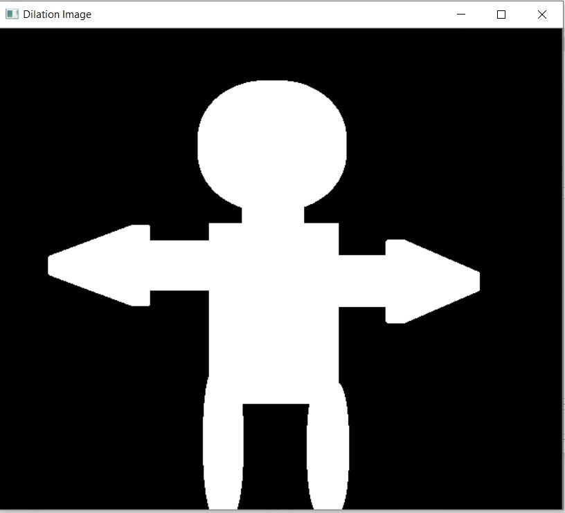
See the black holes/gaps are gone. You will find a combination of erosion and dilation used across many image processing applications.
Working with Videos:
We have learned how to deal with images in OpenCV, now let’s work with Videos in OpenCV. First, it should be clear to you that any operation you perform on images can be done on videos too since a video is nothing but a series of images, for e.g. Consider a 30 FPS video, which means this video shows 30 Frames (images) each second.
There are multiple ways to work with images in OpenCV, you first you have to initialize the camera Object by doing this:
Now there are 4 ways we can use the videoCapture Object depending what you pass in as arg:
1. Using Live camera feed: You pass in an integer number i.e. 0,1,2 etc e.g. cap = cv2.VideoCapture(0), now you will be able to use your webcam live stream.
2. Playing a saved Video on Disk: You pass in the path to the video file e.g. cap = cv2.VideoCapture(Path_To_video).
3. Live Streaming from URL using Ip camera or similar: You can stream from a URL e.g. cap = cv2.VideoCapture(protocol://host:port/script_name?script_params|auth) Note, that each video stream or IP camera feed has its own URL scheme.
4. Read a sequence of Images: You can also read sequences of images but this is not used much.
The next step After Initializing is read from video frame by frame, we do this by using cap.read().
- ret:: A boolean variable which either returns True if the frame was successfully read otherwise False if it fails to read the next frame, this is a really important param when working with videos since after reading the last frame from the video this parameter will return false meaning it can’t read the next frame so we know we can exit the program now.
- frame: This will be a frame/image of our video. Now everytime we run cap.read() it will give us a new frame so we will put cap.read() in a loop and show all the frames sequentially , it will look like we are playing a video but actually we are just displaying frame by frame.
After exiting the loop there is one last thing you must do, you must release the cap object you created by doing cap.release() otherwise your camera will stay on even after the program ends. You may also want to destroy any remaining windows after the loop.
# Initialize Video capture Object.
cap = cv2.VideoCapture(0)


# Initialize a loop in which we will read video frame by frame
while(True):

    # Read frame by frame
    ret, frame = cap.read()

    # If a frame is not read correctly exit the loop, most useful when working with videos on disk
    if not ret:
        break

    # Now we can perform any image processing operations.
    # I’m just going to convert to grayscale and call it a day for this one.
    gray = cv2.cvtColor(frame, cv2.COLOR_BGR2GRAY)

    # Show the frame we just read
    cv2.imshow('frame',gray)

    # Wait for the 1 millisecond, before showing the next frame.
    #  If the user presses the `q` key then exit the loop.
    if cv2.waitKey(1)  ==  ord('q'):
        break

# Release the camera
cap.release()

# Destroy the windows you created
cv2.destroyAllWindows()
Line 2: Initializing the VideoCapture object, if you’re using a usb cam then this value can be 1, 2 etc instead of 0
Line 6-17: looping and reading frame by frame from the camera, making sure it’s not corrupted and then converting to grayscale.
Line 24-25: Check if the user presses the q under 1 millisecond after the imshow function, if yes then exit the loop. The ord() method converts a character to its ASCII value so we can compare it with the returned ASCII value of waitKey() method.
Line 28: Release the camera otherwise your cameras will be left on and the program will exit, this will cause problems the next time you run this cell.
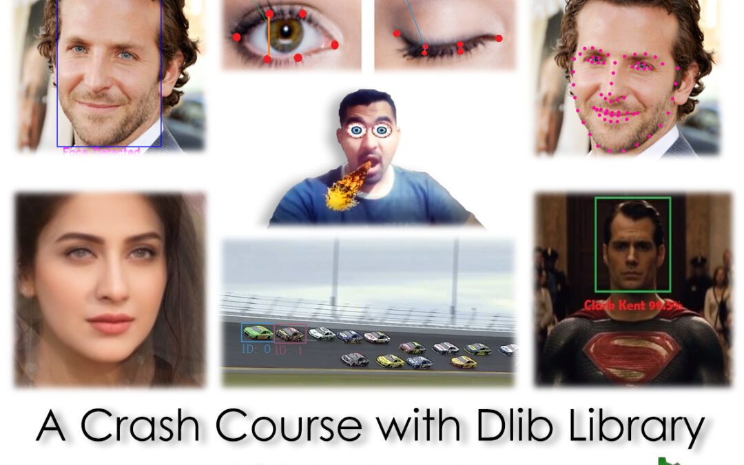
Face Detection with Machine Learning:
In this section we will work with a machine learning-based face detection model, the model we are going to use is a Haar cascade based face detector. It’s the oldest known face detection technique that is still used today at some capacity, although there are more effective approaches, for e.g. take a look at Bleedfacedetector, a python library that I built a year back. It lets users use 4 different types of face detectors by just changing a single line of code.
This Haar Classifier has been trained on several positive (images with faces) and negative (images without faces) images. After training it has learned to recognize faces.
Before using the face detector, you first must initialize it.
cv2.CascadeClassifier(xml_model_file)
- xml_model_file: This is your trained haar cascade model in a .xml file
Detected_faces = cv2.CascadeClassifier.detectMultiScale( image, [ scaleFactor], [minNeighbors])
Params:
- Image: This is your input image.
- scaleFactor: Parameter specifying how much the image size is reduced at each pyramid scale.
- minNeighbors: Parameter specifying how many neighbors each candidate rectangle should have to retain it.
I’m not going to go into the details of this classifier so you can ignore the definitions of scaleFactor & minNeighbors and just remember that you should tune the value of scaleFactor for controlling speed/accuracy tradeoff. Also increase the number of minNeihbors if you’re getting lots of false detections. There is also a minSize & a maxSize parameter which I’m not discussing for now.
Let’s detect all the faces in this image.

# Read the image on which we want to apply face detection
image = cv2.imread('john.jpg')

# Initialize the haar classifier with the face detector model
face_cascade = cv2.CascadeClassifier('haarcascade_frontalface_default.xml')

# Perform the detection, here we are will use 1.3 scale factor and 5 min neighbours
faces = face_cascade.detectMultiScale(image, 1.3, 5)

# Loop through each face and a rectangle on the face coordinates.
for (x,y,w,h) in faces_2:
    cv2.rectangle(img_detection_2,(x,y),(x+w,y+h),(0,255,255),4)
    cv2.putText(img_detection_2,'Face Detected',(x,y+h+15), cv2.FONT_HERSHEY_SIMPLEX, 0.5, (255,0,25), 1, cv2.LINE_AA)


# Display images
cv2.imshow("Original",image);
cv2.imshow("Face Detected",img_detection);
cv2.waitKey(0)
cv2.destroyAllWindows()
Line 8: We are performing face detection and obtaining a list of faces.
Line 11-13: Looping through each face in the list & drawing a rectangle using its coordinates on the image.The list of faces is an array, of x,y,w,h coordinates so an Object (face) is represented as 4 numbers, x,y is the top left corner of the object (face) and w,h is the width and height of the object (face). We can easily use these coordinates to draw a rectangle on the face.
Output:

As you can see almost all faces were detected in the above image. Normally you don’t make deductions regarding a model based on a single image but if I were to make one then I’d say this model is racist or in ML terms this model is biased towards white people.
One issue with these cascades is that they will fail when the face is rotated or is tilted sideways or occupied but no worries you can use a stronger SSD based face detection using bleedfacedetecor.
There are also other Haar Cascades besides this face detector that you can use, take a look at the list here. Not all of them are good but you should try the eye & pedestrian cascades.
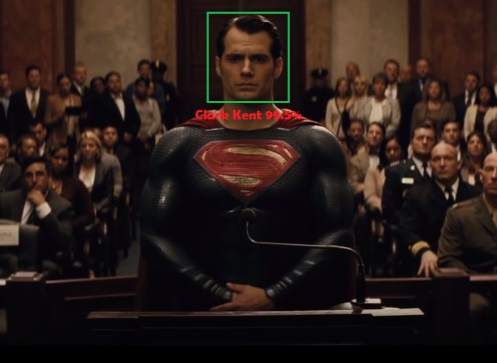
Image Classification with Deep Learning:
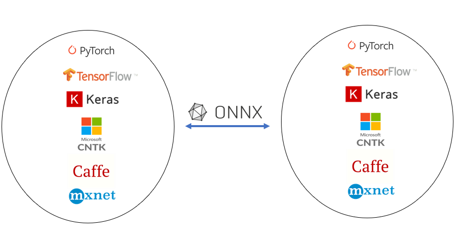
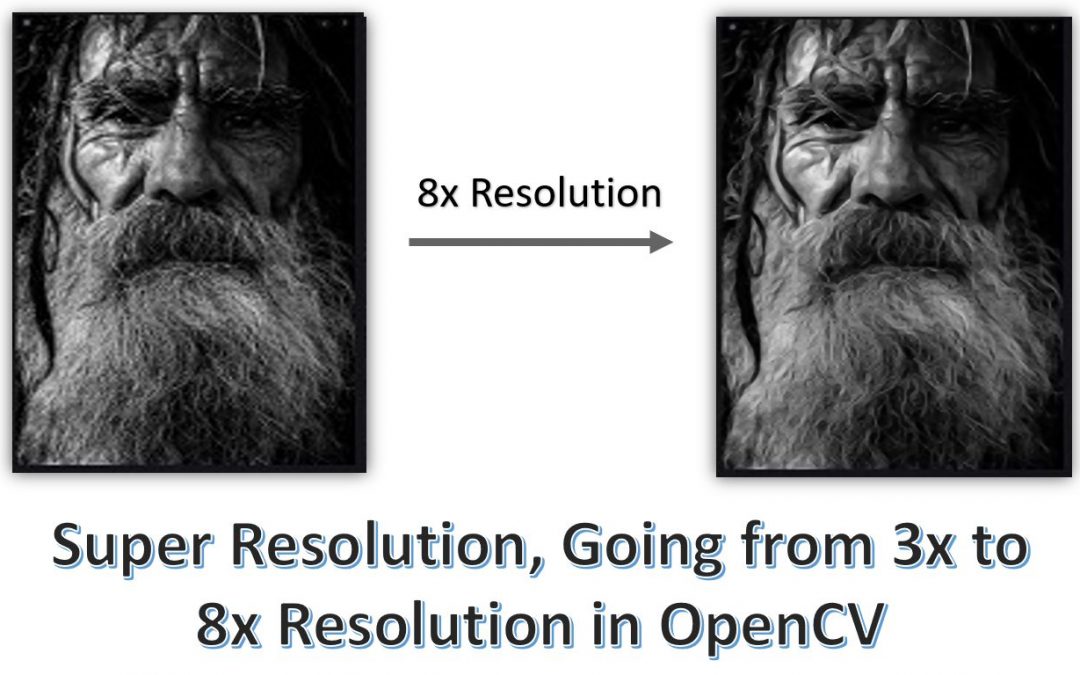
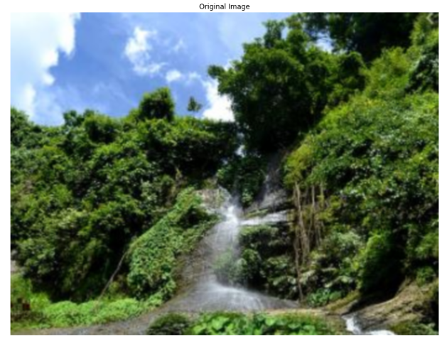
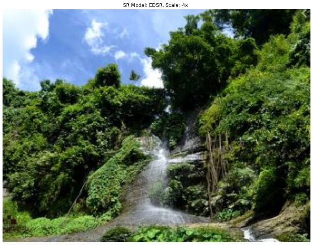
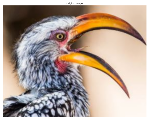
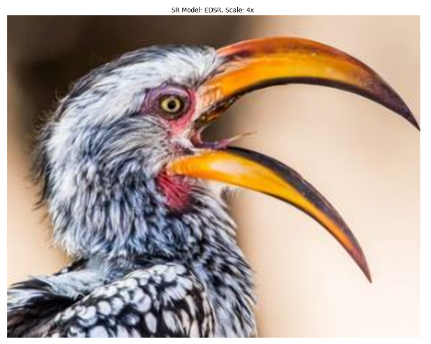
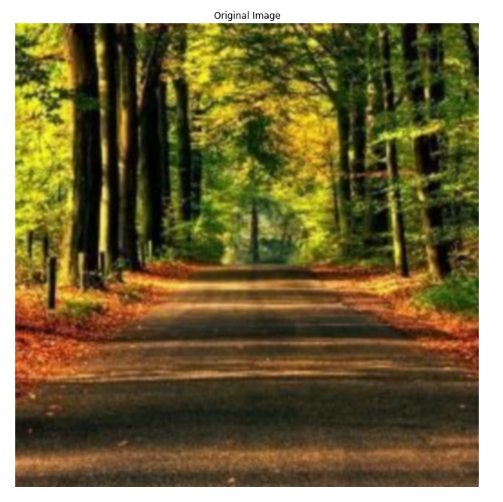
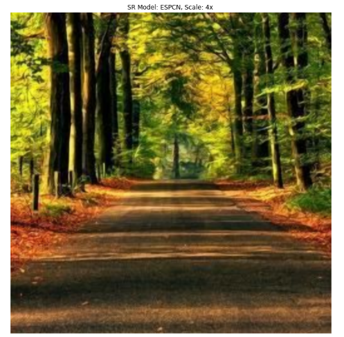
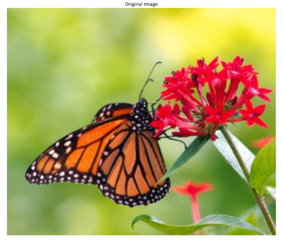
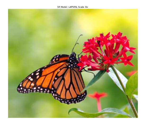
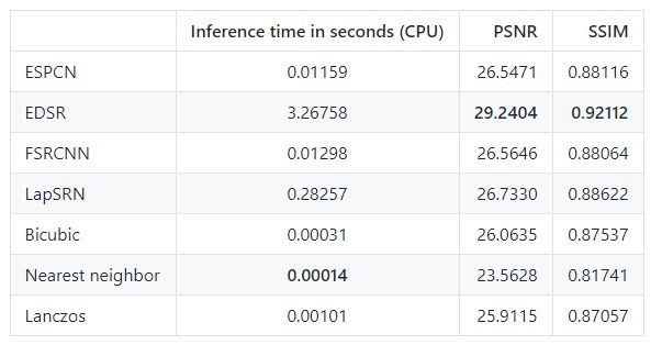
In this section, we will learn to use an image Classifier in OpenCV. We will be using OpenCV’s built-in DNN module. Recently I made a tutorial on performing Super Resolution with DNN module. The DNN module allows you to use pre-trained neural networks from popular frameworks like TensorFlow, PyTorch, ONNX etc. and use those models directly in OpenCV. One problem is that the DNN module does not allow you to train neural networks. Still, it’s a powerful tool, let’s take a look at an image classification pipeline using OpenCV.
Note: I will create a detailed post on OpenCV DNN module in a few weeks, for now I’m keeping this short.
DNN Pipeline
Generally there are 4 steps when doing deep learning with DNN module.
- Read the image and the target classes.
- Initialize the DNN module with an architecture and model parameters.
- Perform the forward pass on the image with the module
- Post process the results.
Now for this we are using a couple of files, like the class labels file, the neural network model and its configuration file, all these files can be downloaded in the source code download section of this post.
We will start by reading the text file containing 1000 ImageNet Classes, and we extract and store each class in a python list.
# Split all the classes by a new line and store it in a variable called rows.
rows = open('synset_words.txt').read().strip().split("n")

# Check the number of classes.
print("Number of Classes "+str(len(rows)))
Output:
Number of Classes 1000
# Show the first 5 rows
print(rows[0:5])
Output:
[‘n01440764 tench, Tinca tinca’, ‘n01443537 goldfish, Carassius auratus’, ‘n01484850 great white shark, white shark, man-eater, man-eating shark, Carcharodon carcharias’, ‘n01491361 tiger shark, Galeocerdo cuvieri’, ‘n01494475 hammerhead, hammerhead shark’]
All these classes are in the text file named synset_words.txt. In this text file, each class is in on a new line with its unique id, Also each class has multiple labels for e.g look at the first 3 lines in the text file:
- ‘n01440764 tench, Tinca tinca’
- ‘n01443537 goldfish, Carassius auratus’
- ‘n01484850 great white shark, white shark
So for each line we have the Class ID, then there are multiple class names, they all are valid names for that class and we’ll just use the first one. So in order to do that we’ll have to extract the second word from each line and create a new list, this will be our labels list.
Here we will extract the labels (2nd element from each line) and create a labels list.
# Split by comma after the first space is found, grab the first element and store it in a new list.
CLASSES = [r[r.find(" ") + 1:].split(",")[0] for r in rows]

# Print the first 50 processed class labels
print(CLASSES[0:50])
Output:
[‘tench’, ‘goldfish’, ‘great white shark’, ‘tiger shark’, ‘hammerhead’, ‘electric ray’, ‘stingray’, ‘cock’, ‘hen’, ‘ostrich’, ‘brambling’, ‘goldfinch’, ‘house finch’, ‘junco’, ‘indigo bunting’, ‘robin’, ‘bulbul’, ‘jay’, ‘magpie’, ‘chickadee’, ‘water ouzel’, ‘kite’, ‘bald eagle’, ‘vulture’, ‘great grey owl’, ‘European fire salamander’, ‘common newt’, ‘eft’, ‘spotted salamander’, ‘axolotl’, ‘bullfrog’, ‘tree frog’, ‘tailed frog’, ‘loggerhead’, ‘leatherback turtle’, ‘mud turtle’, ‘terrapin’, ‘box turtle’, ‘banded gecko’, ‘common iguana’, ‘American chameleon’, ‘whiptail’, ‘agama’, ‘frilled lizard’, ‘alligator lizard’, ‘Gila monster’, ‘green lizard’, ‘African chameleon’, ‘Komodo dragon’, ‘African crocodile’]
Now we will initialize our neural network which is a GoogleNet model trained in a caffe framework on 1000 classes of ImageNet. We will initialize it using cv2.dnn.readNetFromCaffe(), there are different initialization methods for different frameworks.
# This is our model weights file
weights = 'media/bvlc_googlenet.caffemodel'

# This is our model architecture file
architecture ='media/bvlc_googlenet.prototxt'

# Here we will read a pre-trained caffe model with its architecture
net = cv2.dnn.readNetFromCaffe(architecture, weights)
This is the image upon which we will run our classification.

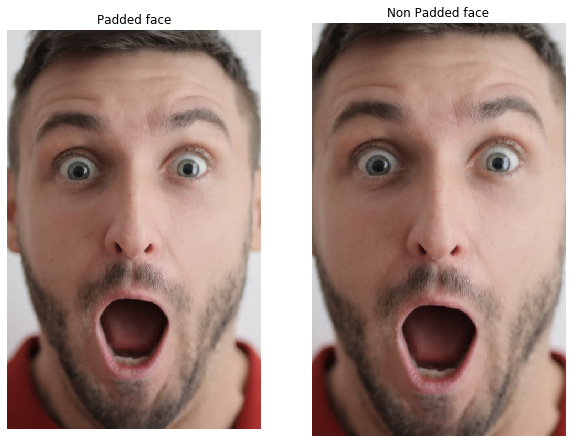
Pre-processing the image:
Now before you pass an image in the network you need to preprocess it, this means resizing the image to the size it was trained on, for many neural networks this is 224x224, in pre-processing step you also do other things like Normalize the image (make the range of intensity values between 0-1) and mean subtraction, etc. These are all the steps the authors did on the images that were used during model training.
Fortunately In OpenCV you have a function called cv2.dnn.blobFromImage() which most of the time takes care of all the pre-processing for you.
blob = cv2.dnn.blobFromImage(image[, scalefactor, [ size], [ mean])
Parameters:
- Image: Input image.
- Scalefactor: Used to normalize the image. This value is multiplied by the image, value of 1 means no scaling is done.
- Size: The size to which the image will be resized to, this depends upon each model.
- Mean: These are mean
R,G,BChannel values from the whole dataset and these are subtracted from the image’sR,G,Bchannels respectively, this gives illumination invariance to the model.
There are other important parameters too but I’m skipping them for now.
# Read the image
image = cv2.imread('media/fish.jpg', 1)

# Pre-process the image, with these values.
blob = cv2.dnn.blobFromImage(image, 1, (224, 224), (104, 117, 123))


# Pass the blob as input through the network
net.setInput(blob)
Now this blob is our pre-processed image. It’s ready to be sent to the network but first you must set it as input
# Pass the blob as input through the network
net.setInput(blob)
This is the most important step, now the image will go through the entire network and you will get an output. Most of the computation time will take place in this step.
# Perform the forward pass
Output = net.forward()
Now if we check the size of Output predictions, we will see that it’s 1000. So the model has returned a list of probabilities for each of the 1000 classes in ImageNet dataset. The index of the highest probability is our target class index.
# Length of the number of predictions
print("Total Number of Predictions are: {}".format(len(Output[0])))
Output:
Total Number of Predictions are: 1000
You can try to print the predictions to understand it better, so we will print initial 50 predictions.
print(Output[0][:50])
Output:
[9.21621759e-05 9.98483717e-01 5.40040501e-09 4.63205048e-08
1.46981725e-08 9.53976155e-07 1.41102263e-09 9.43037321e-07
1.11432279e-07 3.47782636e-11 1.09528010e-07 2.49071910e-08
4.35386397e-07 1.09613385e-09 8.02263755e-10 5.40932188e-09
2.00020311e-09 6.00099359e-10 5.15557423e-11 4.74516648e-10
8.58448729e-11 1.90391162e-07 3.05192899e-10 1.51088759e-08
1.51897750e-09 6.16360580e-07 5.98882507e-05 1.80176867e-04
1.07785991e-06 2.55477469e-04 1.88719014e-07 5.45302964e-06
2.64027094e-05 2.53552770e-07 5.08395566e-08 6.60280875e-07
1.89136574e-06 8.86267983e-08 5.25031763e-04 3.21334414e-06
6.80627727e-06 2.47660046e-06 1.29753553e-05 1.73194076e-06
1.06492757e-06 3.31227341e-07 1.72065847e-06 4.86000363e-06
3.48621292e-08 1.47009416e-07]
Now if I wanted to get the top most prediction or the highest probability then we would just need to do np.max()
# Maximum probability
print(np.max(Output[0]))
Output:
0.9984837
See, we got a class with 99.84% probability. This is really good, it means our network is pretty sure about the name of the target class.
If we wanted to check the index of the target class we can just do np.argmax()
# Index of Class with the maximum Probability.
index = np.argmax(Output[0])
print(index)
Output:
1
Our network says the class with the highest probability is at index 1. We just have to use this index in the labels list to get the name of the actual predicted class.
print(CLASSES[index])
Output:
goldfish
So our target class is goldfish which has a probability of 99.84%
In the final step we are just going to put the above information over the image.
# Create text that says the class name and its probability.
text = "Label: {}, {:.2f}%".format(CLASSES[index], np.max(Output[0]))

# Put the text on the image
cv2.putText(image, text, (20, 20 ),  cv2.FONT_HERSHEY_COMPLEX, 1, (100, 20, 255), 2)

# Display image
cv2.imshow("Classified Image",image);
cv2.waitKey(0)
cv2.destroyAllWindows()
Output:
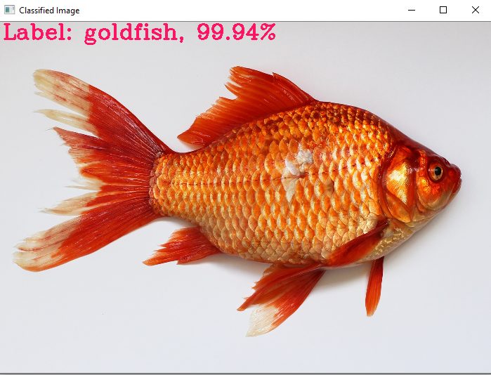
So this was an Image classification pipeline, similarly there are a lot of other interesting neural nets for different tasks, Object Detection, Image Segmentation, Image Colorization etc. I cover using 13-14 Different Neural nets with OpenCV using Video Walkthroughs and notebooks inside our Computer Vision Course and also show you how to use them with Nvidia & OpenCL GPUs.
What’s Next?
If you want to go forward from here and learn more advanced things and go into more detail, understand theory and code of different algorithms then be sure to check out our Computer Vision & Image Processing with Python Course (Urdu/Hindi). In this course I go into a lot more detail on each of the topics that I’ve covered above.
If you want to start a career in Computer Vision & Artificial Intelligence then this course is for you. One of the best things about this course is that the video lectures are in Urdu/Hindi Language without any compromise on quality, so there is a personal/local touch to it.
Summary:
In this post, we covered a lot of fundamentals in OpenCV. We learn to work with images as well as videos, this should serve as a good starting point but keep on learning. Remember to refer to OpenCV documentation and StackOverflow if you’re stuck on something. In a few weeks, I’ll be sharing our Computer Vision Resource Guide, which will help you in your Computer Vision journey.
If you have any questions or confusion regarding this post, feel free to comment on this post and I’ll be happy to help.
You can reach out to me personally for a 1 on 1 consultation session in AI/computer vision regarding your project. Our talented team of vision engineers will help you every step of the way. Get on a call with me directly here.