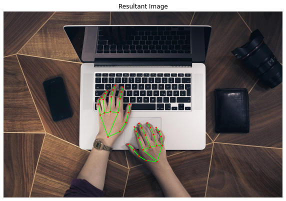
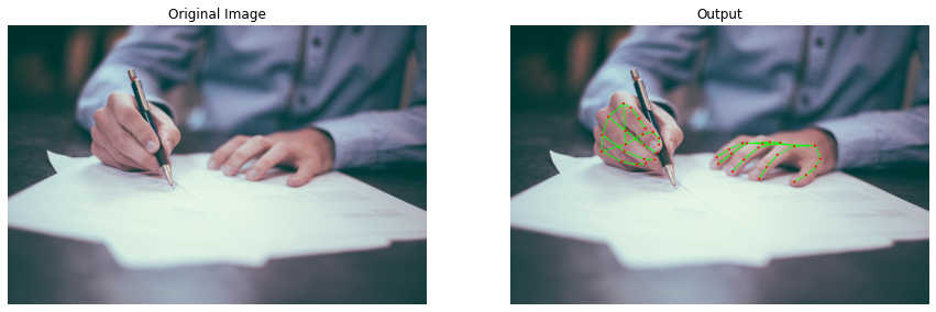
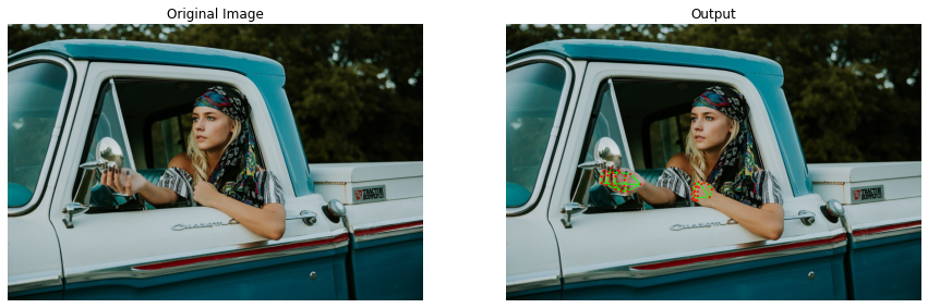
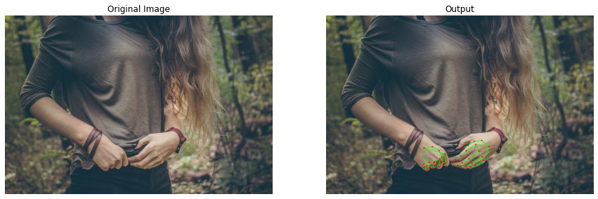
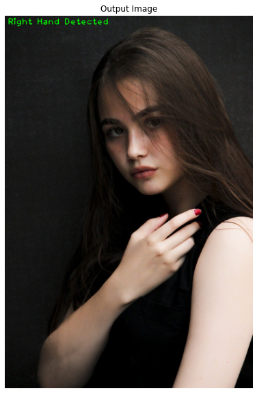
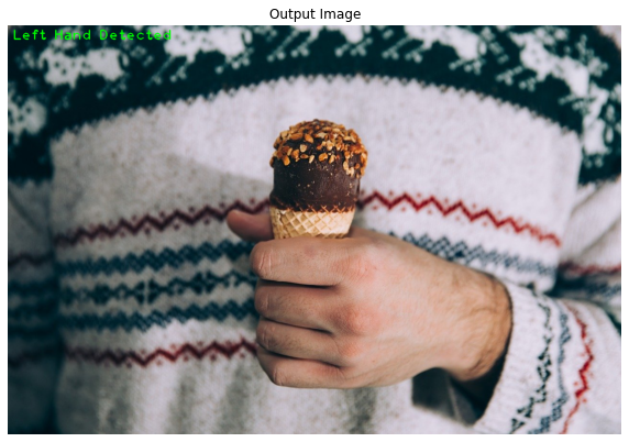
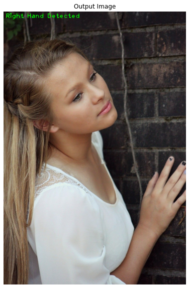
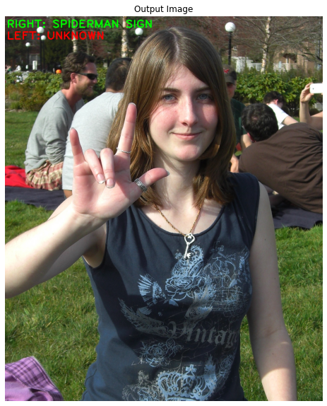
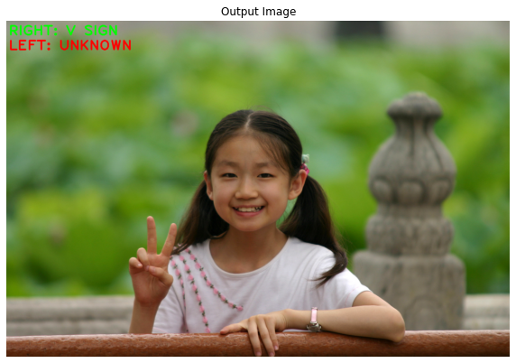
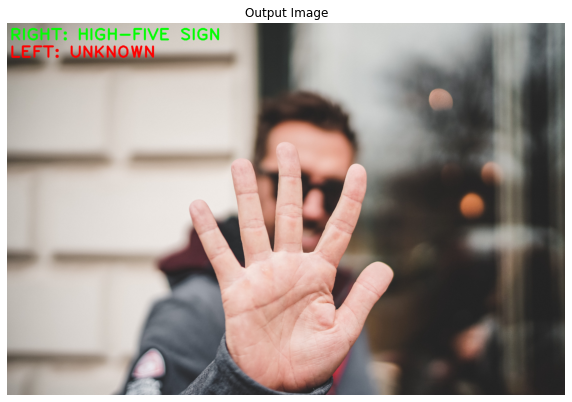
In this tutorial, we’ll learn how to do real-time 3D hands landmarks detection using the Mediapipe library in python. After that, we’ll learn to perform hands type classification (i.e. is it a left or right hand) and then draw the bounding boxes around the hands by retrieving the required coordinates from the detected landmarks.
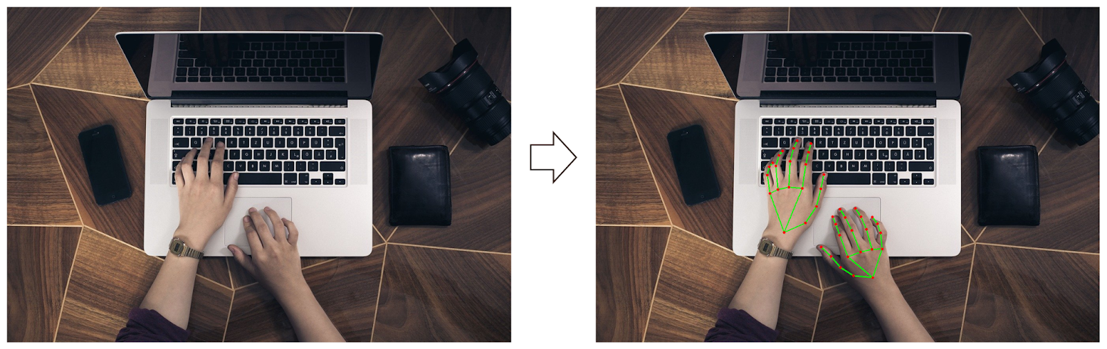
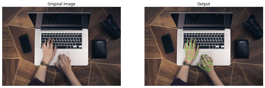
Below are the results on a few sample images, and this will work on real-time camera feed or recorded videos as well.
And last but not the least, we will also create a customized landmarks annotation of the hands utilizing the depth (distance from the camera) of the hands, as Mediapipe’s solution provides three-dimensional landmarks.
The annotation provided by Mediapipe allows users to annotate the images and videos with a single line of code but it does not utilize the depth and draws fixed-sized lines and circles on the hands.
But in our customized annotation, the thickness of the lines (connections) and circles (landmarks) for each hand will vary in real-time by using the depth of each hand, with the decrease in the distance from the camera (depth), the size of the annotation increases.
The motivation behind this was that the size of the hand in the image/frame increases when the hand is moved closer to the camera, so using a fixed size annotation for a hand that varies in size was hard to digest for me. You can see the comparison of Mediapipe’s annotation and our customized annotation below.
The code for all this is very easy and is explained in the simplest manner possible.
Now before diving further, you can go and watch the youtube tutorial for the detailed explanation, although this blog post alone can also serve the purpose.
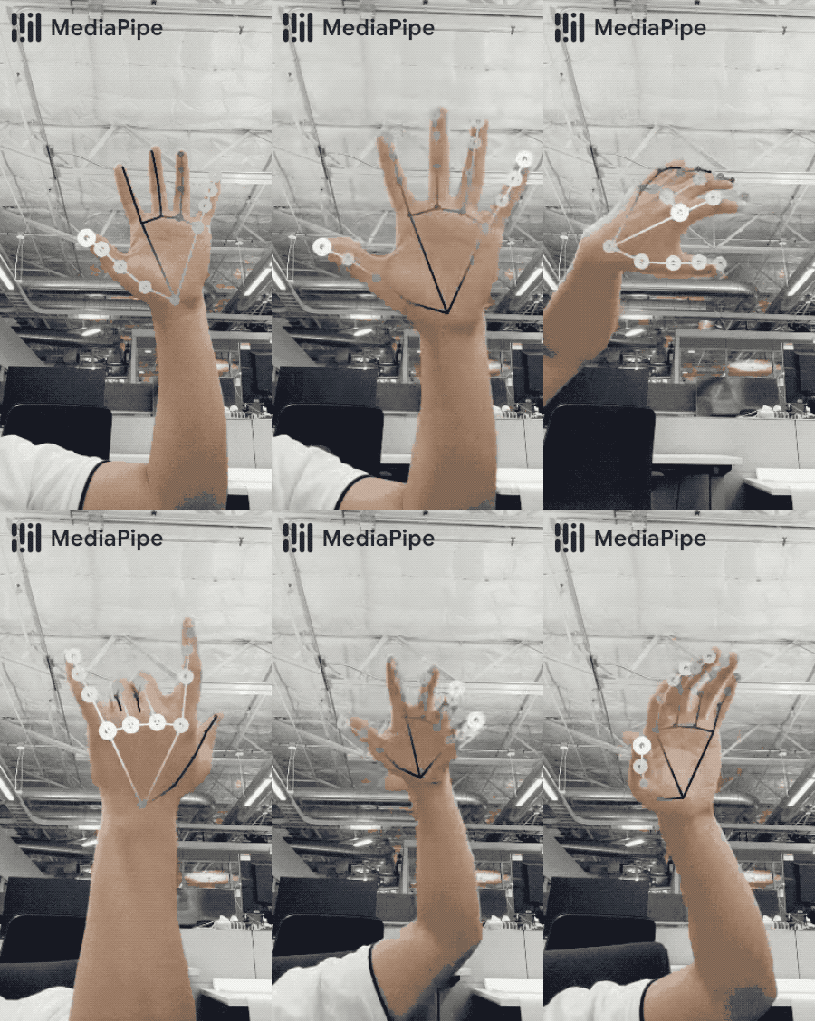
In this one, we will learn to localize twenty-one key landmarks on hand(s) e.g. wrist, thumb and fingertips, etc. See the image below:
It is an important and popular pre-processing task in many vision applications as it allows to localize and recognize the shape and motion of hands that opens up the door to the future by making a ton of applications feasible like:
Augmented Reality Applications that overlay Digital Content and Information over Reality like a Virtual Painter.
Sign Language Recognition.
Hand Gesture Controlled Drones and Robots or any other Physical Appliances.
Using landmark detection is also a great way to interact with any Human-Computer Interaction (HCI) based system as the human hand is capable of making multiple gestures without much effort.
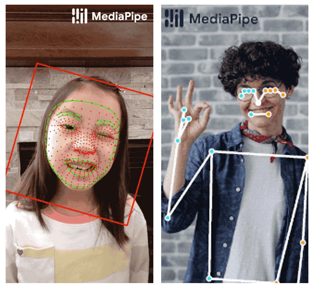
Some other types of keypoint detection problems are facial landmark detection, pose detection, etc.
I have already made a tutorial on pose detection and will explain facial landmark detection in an upcoming tutorial.
Part 1 (b): Mediapipe’s Hands Landmarks Detection Implementation
Here’s a brief introduction to Mediapipe;
“Mediapipe is a cross-platform/open-source tool that allows you to run a variety of machine learning models in real-time. It’s designed primarily for facilitating the use of ML in streaming media & It was built by Google”
All the models in Mediapipe have state-of-the-art performance and are highly optimized as well and are used in a lot of well-known products out there.
It provides a robust solution capable of predicting twenty-one 3D landmarks on a hand in real-time with high accuracy and speed as well, even on low-end devices i.e. phones, laptops, etc., which makes it stand out from the other solutions out there.
Now you may be thinking what makes it so fast?
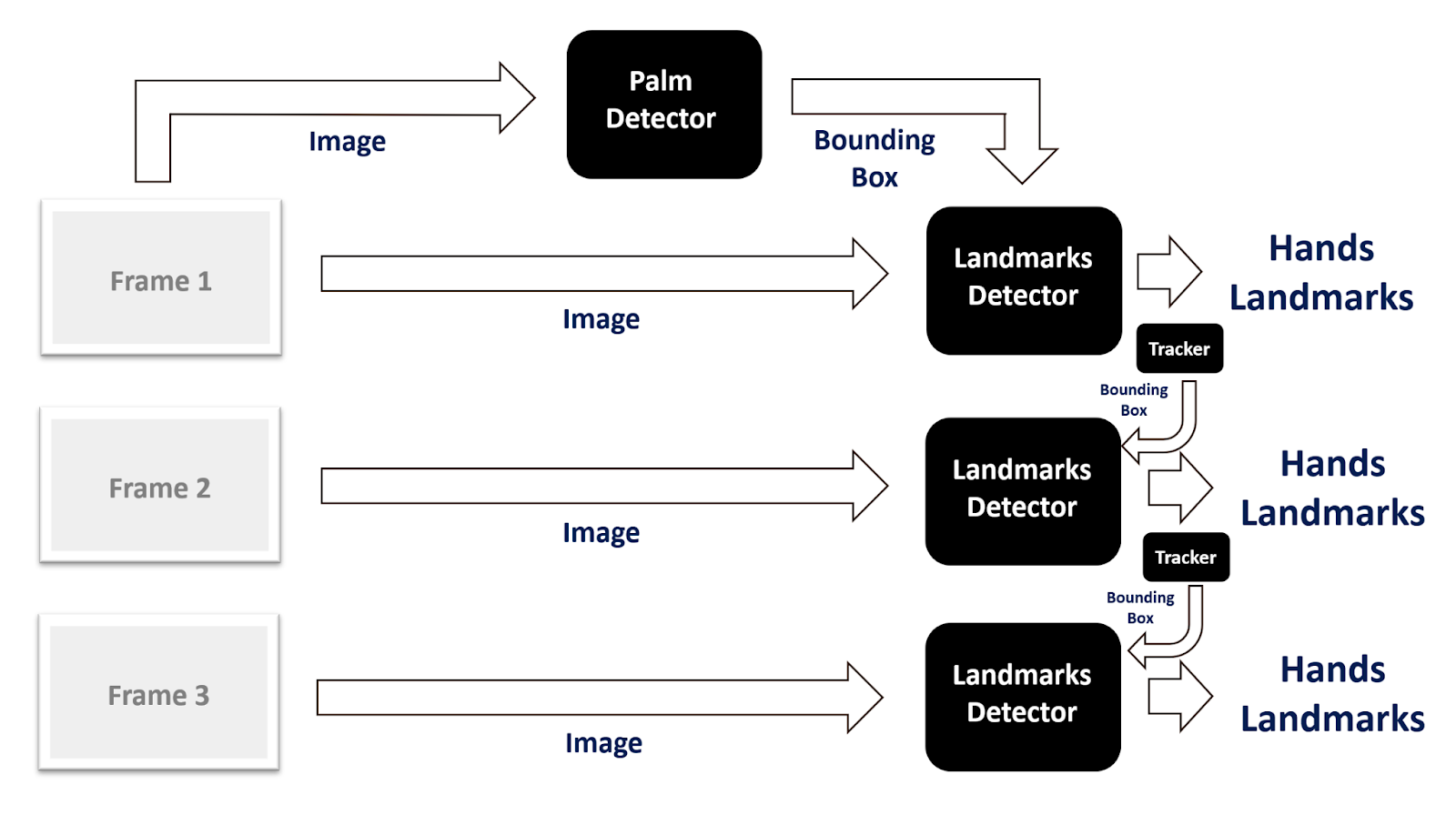
Actually, they have combined a computationally costly object detector with an object tracker that requires a lot less processing. So for the videos, a tracker is used instead of invoking the object detector at every frame which makes this solution so fast and brilliant.
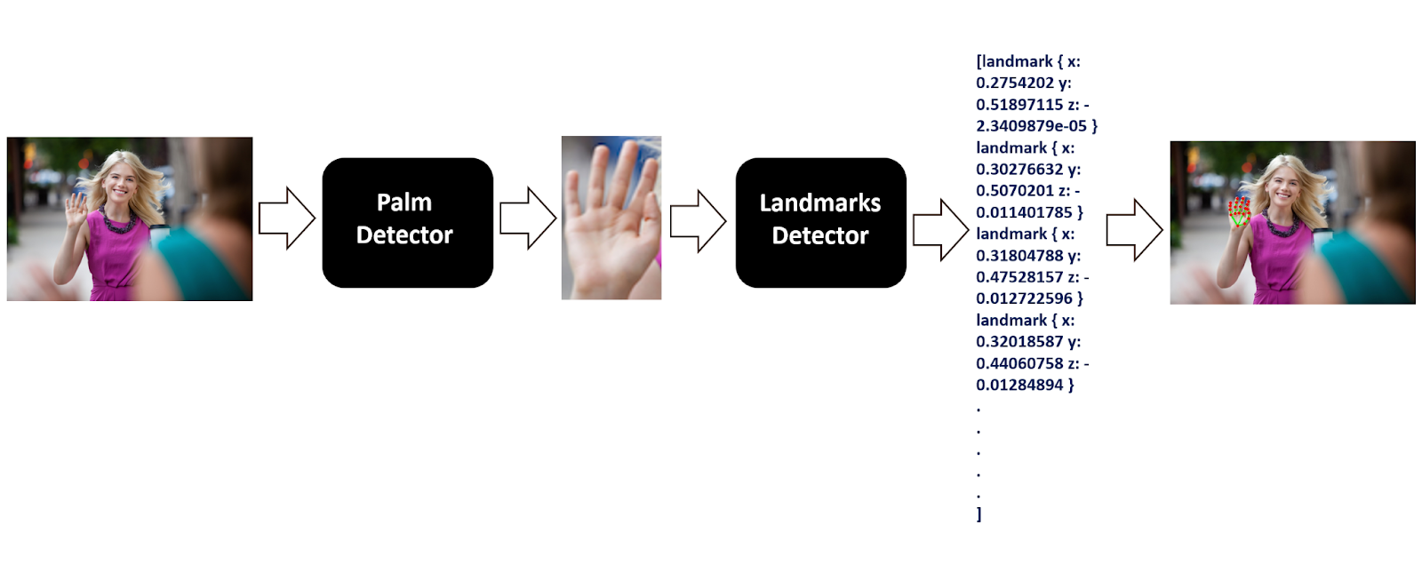
The detector is only invoked as needed, that is in the very first frame or when the tracker loses track of any of the hands. The detector localizes the hand in the image/frame and outputs the bounding box coordinates around the hand.
Then the region of interest (ROI) is cropped from the image/frame using the bounding box coordinates and after that, the cropped image/frame is used by the hand landmark model to predict the landmarks within the ROI.
The palm detector is used, as detecting hands is a comparatively more complex task than the palm or fist (i.e., rigid objects). Palms require square bounding boxes which reduces the number of anchors (predefined bounding boxes of a certain height and width). Also as palms are smaller objects, which reduces the possibility of self-occlusion (hidden by themselves), like handshakes. Comparatively, hands lack easily distinguishable patterns and are often occluded.
The image below shows the twenty-one hand landmarks, that this solution detects, along with their indexes.
They manually annotated around 30K real-world images with 3D coordinates by using images depth maps and also rendered a high-quality synthetic hand model over various backgrounds and then mapped the model with different backgrounds to the corresponding 3D coordinates.
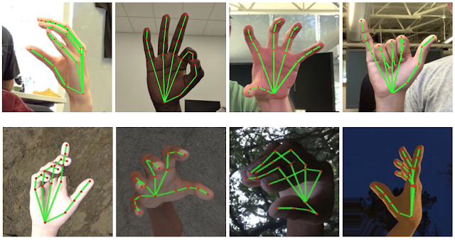
So they kind of automated the whole annotation process. The image below contains the aligned hands cropped images and the rendered synthetic hand images with ground truth annotation.
Alright now we have learned the required basic theory and implementation details, let’s dive into the code.
Download Code:
[optin-monster slug=”ko5ox1sveedosrhdesgq”]
Import the Libraries
We will start by importing the required libraries.
import cv2
import numpy as np
from time import time
import mediapipe as mp
import matplotlib.pyplot as plt
Part 2: Using Hands Landmarks Detection on images and videos
Initialize the Hands Landmarks Detection Model
To use the Mediapipe’s hands solution, we first have to initialize the hands class using the mp.solutions.hands syntax and then we will have to call the function mp.solutions.hands.Hands() with the arguments explained below:
static_image_mode – It is a boolean value that is if set to False, the solution treats the input images as a video stream. It will try to detect hands in the first input images, and upon a successful detection further localizes the hand landmarks. In subsequent images, once all max_num_hands hands are detected and the corresponding hand landmarks are localized, it simply tracks those landmarks without invoking another detection until it loses track of any of the hands. This reduces latency and is ideal for processing video frames. If set to True, hand detection runs on every input image, ideal for processing a batch of static, possibly unrelated, images. Its default value is False.
max_num_hands – It is the maximum number of hands to detect. Its default value is 2.
min_detection_confidence – It is the minimum detection confidence ([0.0, 1.0]) required to consider the palm-detection model’s prediction correct. Its default value is 0.5 which means that all the detections with prediction confidence less than 50% are ignored by default.
min_tracking_confidence – It is the minimum tracking confidence ([0.0, 1.0]) required to consider the landmark-tracking model’s tracked hands landmarks valid. If the confidence is less than this argument value then the detector is invoked again in the next frame/image, so increasing its value increases the robustness, but also increases the latency. Its default value is 0.5.
Then we will also need to initialize the mp.solutions.drawing_utils class that is very useful to visualize the landmarks on the images/frames.
# Initialize the mediapipe hands class.
mp_hands = mp.solutions.hands

# Set up the Hands function.
hands = mp_hands.Hands(static_image_mode=True, max_num_hands=2, min_detection_confidence=0.3)

# Initialize the mediapipe drawing class.
mp_drawing = mp.solutions.drawing_utils
Read an Image
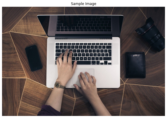
Now we will use the function cv2.imread() to read a sample image and then display it using the matplotlib library.
# Read an image from the specified path.
sample_img = cv2.imread('media/sample.jpg')

# Specify a size of the figure.
plt.figure(figsize = [10, 10])

# Display the sample image, also convert BGR to RGB for display.
plt.title("Sample Image");plt.axis('off');plt.imshow(sample_img[:,:,::-1]);plt.show()
Perform Hands Landmarks Detection
Now we will pass the image to the hand’s landmarks detection machine learning pipeline by using the function mp.solutions.hands.Hands().process(). But first, we will have to convert the image from BGR to RGB format using the function cv2.cvtColor() as OpenCV reads images in BGR format and the ml pipeline expects the input images to be in RGB color format.
The machine learning pipeline outputs a list of twenty-one landmarks of the prominent hands in the image. Each landmark has:
x – It is the landmark x-coordinate normalized to [0.0, 1.0] by the image width.
y: It is the landmark y-coordinate normalized to [0.0, 1.0] by the image height.
z: It is the landmark z-coordinate normalized to roughly the same scale as x. It represents the landmark depth with the wrist being the origin, so the smaller the value the closer the landmark is to the camera.
To get more intuition, we will display the first two landmarks of each hand, the ml pipeline outputs an object that has an attribute multi_hand_landmarks that contains the found landmarks coordinates of each hand as an element of a list.
Note:The z-coordinate is just the relative distance of the landmark from the wrist, and this distance increases and decreases depending upon the distance from the camera so that is why it represents the depth of each landmark point.
# Perform hands landmarks detection after converting the image into RGB format.
results = hands.process(cv2.cvtColor(sample_img, cv2.COLOR_BGR2RGB))

# Check if landmarks are found.
if results.multi_hand_landmarks:

    # Iterate over the found hands.
    for hand_no, hand_landmarks in enumerate(results.multi_hand_landmarks):

        print(f'HAND NUMBER: {hand_no+1}')
        print('-----------------------')

        # Iterate two times as we only want to display first two landmarks of each hand.
        for i in range(2):

            # Display the found normalized landmarks.
            print(f'{mp_hands.HandLandmark(i).name}:')
            print(f'{hand_landmarks.landmark[mp_hands.HandLandmark(i).value]}')
As you can see that the landmarks are normalized to specific scales, so now we will convert them back to their original scale by using the width and height of the sample image and display them.
# Retrieve the height and width of the sample image.
image_height, image_width, _ = sample_img.shape

# Check if landmarks are found.
if results.multi_hand_landmarks:

    # Iterate over the found hands.
    for hand_no, hand_landmarks in enumerate(results.multi_hand_landmarks):

        print(f'HAND NUMBER: {hand_no+1}')
        print('-----------------------')

        # Iterate two times as we only want to display first two landmark of each hand.
        for i in range(2):

            # Display the found landmarks after converting them into their original scale.
            print(f'{mp_hands.HandLandmark(i).name}:')
            print(f'x: {hand_landmarks.landmark[mp_hands.HandLandmark(i).value].x * image_width}')
            print(f'y: {hand_landmarks.landmark[mp_hands.HandLandmark(i).value].y * image_height}')
            print(f'z: {hand_landmarks.landmark[mp_hands.HandLandmark(i).value].z * image_width}\n')
Now we will draw the detected landmarks on a copy of the sample image using the function mp.solutions.drawing_utils.draw_landmarks() from the class mp.solutions.drawing_utils, we had initialized earlier and will display the resultant image.
# Create a copy of the sample image to draw landmarks on.
img_copy = sample_img.copy()

# Check if landmarks are found.
if results.multi_hand_landmarks:

    # Iterate over the found hands.
    for hand_no, hand_landmarks in enumerate(results.multi_hand_landmarks):

        # Draw the hand landmarks on the copy of the sample image.
        mp_drawing.draw_landmarks(image = img_copy, landmark_list = hand_landmarks,
                                  connections = mp_hands.HAND_CONNECTIONS)

    # Specify a size of the figure.
    fig = plt.figure(figsize = [10, 10])

    # Display the resultant image with the landmarks drawn, also convert BGR to RGB for display.
    plt.title("Resultant Image");plt.axis('off');plt.imshow(img_copy[:,:,::-1]);plt.show()
Part 3: Hands Classification (i.e., Left or Right)
Create a Hands Landmarks Detection Function
Now we will put all this together to create a function that will perform hands landmarks detection on an image and will visualize the resultant image along with the original image or return the resultant image along with the output of the model depending upon the passed arguments.
def detectHandsLandmarks(image, hands, display = True):
    '''
    This function performs hands landmarks detection on an image.
    Args:
        image:   The input image with prominent hand(s) whose landmarks needs to be detected.
        hands:   The hands function required to perform the hands landmarks detection.
        display: A boolean value that is if set to true the function displays the original input image, and the output
                 image with hands landmarks drawn and returns nothing.
    Returns:
        output_image: The input image with the detected hands landmarks drawn.
        results: The output of the hands landmarks detection on the input image.
    '''

    # Create a copy of the input image to draw landmarks on.
    output_image = image.copy()

    # Convert the image from BGR into RGB format.
    imgRGB = cv2.cvtColor(image, cv2.COLOR_BGR2RGB)

    # Perform the Hands Landmarks Detection.
    results = hands.process(imgRGB)

    # Check if landmarks are found.
    if results.multi_hand_landmarks:

        # Iterate over the found hands.
        for hand_landmarks in results.multi_hand_landmarks:

            # Draw the hand landmarks on the copy of the input image.
            mp_drawing.draw_landmarks(image = output_image, landmark_list = hand_landmarks,
                                  connections = mp_hands.HAND_CONNECTIONS)

    # Check if the original input image and the output image are specified to be displayed.
    if display:

        # Display the original input image and the output image.
        plt.figure(figsize=[15,15])
        plt.subplot(121);plt.imshow(image[:,:,::-1]);plt.title("Original Image");plt.axis('off');
        plt.subplot(122);plt.imshow(output_image[:,:,::-1]);plt.title("Output");plt.axis('off');

    # Otherwise
    else:

        # Return the output image and results of hands landmarks detection.
        return output_image, results
Now we will utilize the function created above to perform hands landmarks detection on a few sample images and display the results.
# Read another sample image and perform hands landmarks detection on it.
image = cv2.imread('media/sample1.jpg')
detectHandsLandmarks(image, hands, display=True)
# Read another sample image and perform hands landmarks detection on it.
image = cv2.imread('media/sample2.jpg')
detectHandsLandmarks(image, hands, display=True)
# Read another sample image and perform hands landmarks detection on it.
image = cv2.imread('media/sample3.jpg')
detectHandsLandmarks(image, hands, display=True)
Hands Landmarks Detection on Real-Time Webcam Feed
The results on the images were excellent, but now the real test begins, we will try the function on a real-time webcam feed. We will also calculate and display the number of frames being updated in one second to get an idea of whether this solution can work in real-time on a CPU or not. As that is the only thing that differentiates it from the other solutions out there.
# Setup Hands function for video.
hands_video = mp_hands.Hands(static_image_mode=False, max_num_hands=2,
                             min_detection_confidence=0.7, min_tracking_confidence=0.4)

# Initialize the VideoCapture object to read from the webcam.
camera_video = cv2.VideoCapture(1)
camera_video.set(3,1280)
camera_video.set(4,960)

# Create named window for resizing purposes.
cv2.namedWindow('Hands Landmarks Detection', cv2.WINDOW_NORMAL)

# Initialize a variable to store the time of the previous frame.
time1 = 0

# Iterate until the webcam is accessed successfully.
while camera_video.isOpened():

    # Read a frame.
    ok, frame = camera_video.read()

    # Check if frame is not read properly then continue to the next iteration to read the next frame.
    if not ok:
        continue

    # Flip the frame horizontally for natural (selfie-view) visualization.
    frame = cv2.flip(frame, 1)

    # Perform Hands landmarks detection.
    frame, _ = detectHandsLandmarks(frame, hands_video, display=False)

    # Set the time for this frame to the current time.
    time2 = time()

    # Check if the difference between the previous and this frame time > 0 to avoid division by zero.
    if (time2 - time1) > 0:

        # Calculate the number of frames per second.
        frames_per_second = 1.0 / (time2 - time1)

        # Write the calculated number of frames per second on the frame.
        cv2.putText(frame, 'FPS: {}'.format(int(frames_per_second)), (10, 30),cv2.FONT_HERSHEY_PLAIN, 2, (0, 255, 0), 3)

    # Update the previous frame time to this frame time.
    # As this frame will become previous frame in next iteration.
    time1 = time2

    # Display the frame.
    cv2.imshow('Hands Landmarks Detection', frame)

    # Wait for 1ms. If a a key is pressed, retreive the ASCII code of the key.
    k = cv2.waitKey(1) & 0xFF

    # Check if 'ESC' is pressed and break the loop.
    if(k == 27):
        break

# Release the VideoCapture Object and close the windows.
camera_video.release()
cv2.destroyAllWindows()
Output
Woah! that was impressive not only it was fast but the results were quite accurate too.
Create a Hand Type Classification Function
Now we will create a function that will perform hands type classification (i.e. is it a left or right hand). The output (object) by the hand’s landmarks detector model contains another attribute multi_handedness that contains a score (probability of the predicted label being correct) and label (either "Left" or "Right") for each detected hand.
While determining the label, it is assumed that the input image is mirrored (i.e., flipped horizontally). So we had already performed classification during the hand’s landmarks detection, and now we only need to access the information stored in the attribute multi_handedness.
def getHandType(image, results, draw=True, display = True):
    '''
    This function performs hands type (left or right) classification on hands.
    Args:
        image:   The image of the hands that needs to be classified, with the hands landmarks detection already performed.
        results: The output of the hands landmarks detection performed on the image in which hands types needs
                 to be classified.
        draw:    A boolean value that is if set to true the function writes the hand type label on the output image.
        display: A boolean value that is if set to true the function displays the output image and returns nothing.
    Returns:
        output_image: The image of the hands with the classified hand type label written if it was specified.
        hands_status: A dictionary containing classification info of both hands.
    '''

    # Create a copy of the input image to write hand type label on.
    output_image = image.copy()

    # Initialize a dictionary to store the classification info of both hands.
    hands_status = {'Right': False, 'Left': False, 'Right_index' : None, 'Left_index': None}

    # Iterate over the found hands in the image.
    for hand_index, hand_info in enumerate(results.multi_handedness):

        # Retrieve the label of the found hand.
        hand_type = hand_info.classification[0].label

        # Update the status of the found hand.
        hands_status[hand_type] = True

        # Update the index of the found hand.
        hands_status[hand_type + '_index'] = hand_index

        # Check if the hand type label is specified to be written.
        if draw:

            # Write the hand type on the output image.
            cv2.putText(output_image, hand_type + ' Hand Detected', (10, (hand_index+1) * 30),cv2.FONT_HERSHEY_PLAIN,
                        2, (0,255,0), 2)

    # Check if the output image is specified to be displayed.
    if display:

        # Display the output image.
        plt.figure(figsize=[10,10])
        plt.imshow(output_image[:,:,::-1]);plt.title("Output Image");plt.axis('off');

    # Otherwise
    else:

        # Return the output image and the hands status dictionary that contains classification info.
        return output_image, hands_status
Now we will utilize the function created above to perform hand type classification on a few sample images and display the results.
# Read a sample image with one hand and perform hand type classification on it after flipping it horizontally.
image = cv2.imread('media/sample5.jpg')
flipped_image = cv2.flip(image, 1)
_, results = detectHandsLandmarks(flipped_image, hands, display=False)
if results.multi_hand_landmarks:
    getHandType(image, results)
# Read a sample image with one hand and perform hand type classification on it after flipping it horizontally.
image = cv2.imread('media/sample6.jpg')
flipped_image = cv2.flip(image, 1)
_, results = detectHandsLandmarks(flipped_image, hands, display=False)
if results.multi_hand_landmarks:
    getHandType(image, results)
# Read a sample image with one hand and perform hand type classification on it after flipping it horizontally.
image = cv2.imread('media/sample7.jpg')
flipped_image = cv2.flip(image, 1)
_, results = detectHandsLandmarks(flipped_image, hands, display=False)
if results.multi_hand_landmarks:
    getHandType(image, results)
Cool! it worked perfectly on each of the sample images.
Part 4 (a): Draw Bounding Boxes around the Hands
Create a Function to Draw Bounding Boxes
Now we will create a function that will draw bounding boxes around the hands and write their classified types near them. We will first convert the normalized landmarks back to their original scale by using the width and height of the image. We will then get the bounding box coordinates ((x1,y1), (x2, y2)) for each hand.
Top Left Coordinate:
x1 – the smallest x-coordinate in the list of the found landmarks of the hand.
y1 – the smallest y-coordinate in the list of the found landmarks of the hand.
Bottom Right Coordinate:
x2 – the largest x-coordinate in the list of the found landmarks of the hand.
y2 – the largest y-coordinate in the list of the found landmarks of the hand.
Then we will draw the bounding boxes around the hands using the found coordinates and the specified padding and write the classified types of each hand near them using the bounding box coordinates. And after that, we will either display the resultant image or return it depending upon the passed arguments.
def drawBoundingBoxes(image, results, hand_status, padd_amount = 10, draw=True, display=True):
    '''
    This function draws bounding boxes around the hands and write their classified types near them.
    Args:
        image:       The image of the hands on which the bounding boxes around the hands needs to be drawn and the
                     classified hands types labels needs to be written.
        results:     The output of the hands landmarks detection performed on the image on which the bounding boxes needs
                     to be drawn.
        hand_status: The dictionary containing the classification info of both hands.
        padd_amount: The value that specifies the space inside the bounding box between the hand and the box's borders.
        draw:        A boolean value that is if set to true the function draws bounding boxes and write their classified
                     types on the output image.
        display:     A boolean value that is if set to true the function displays the output image and returns nothing.
    Returns:
        output_image:     The image of the hands with the bounding boxes drawn and hands classified types written if it
                          was specified.
        output_landmarks: The dictionary that stores both (left and right) hands landmarks as different elements.
    '''

    # Create a copy of the input image to draw bounding boxes on and write hands types labels.
    output_image = image.copy()

    # Initialize a dictionary to store both (left and right) hands landmarks as different elements.
    output_landmarks = {}

    # Get the height and width of the input image.
    height, width, _ = image.shape

    # Iterate over the found hands.
    for hand_index, hand_landmarks in enumerate(results.multi_hand_landmarks):

        # Initialize a list to store the detected landmarks of the hand.
        landmarks = []

        # Iterate over the detected landmarks of the hand.
        for landmark in hand_landmarks.landmark:

            # Append the landmark into the list.
            landmarks.append((int(landmark.x * width), int(landmark.y * height),
                                  (landmark.z * width)))

        # Get all the x-coordinate values from the found landmarks of the hand.
        x_coordinates = np.array(landmarks)[:,0]

        # Get all the y-coordinate values from the found landmarks of the hand.
        y_coordinates = np.array(landmarks)[:,1]

        # Get the bounding box coordinates for the hand with the specified padding.
        x1  = int(np.min(x_coordinates) - padd_amount)
        y1  = int(np.min(y_coordinates) - padd_amount)
        x2  = int(np.max(x_coordinates) + padd_amount)
        y2  = int(np.max(y_coordinates) + padd_amount)

        # Initialize a variable to store the label of the hand.
        label = "Unknown"

        # Check if the hand we are iterating upon is the right one.
        if hand_status['Right_index'] == hand_index:

            # Update the label and store the landmarks of the hand in the dictionary.
            label = 'Right Hand'
            output_landmarks['Right'] = landmarks

        # Check if the hand we are iterating upon is the left one.
        elif hand_status['Left_index'] == hand_index:

            # Update the label and store the landmarks of the hand in the dictionary.
            label = 'Left Hand'
            output_landmarks['Left'] = landmarks

        # Check if the bounding box and the classified label is specified to be written.
        if draw:

            # Draw the bounding box around the hand on the output image.
            cv2.rectangle(output_image, (x1, y1), (x2, y2), (155, 0, 255), 3, cv2.LINE_8)

            # Write the classified label of the hand below the bounding box drawn.
            cv2.putText(output_image, label, (x1, y2+25), cv2.FONT_HERSHEY_COMPLEX, 0.7, (20,255,155), 1, cv2.LINE_AA)

    # Check if the output image is specified to be displayed.
    if display:

        # Display the output image.
        plt.figure(figsize=[10,10])
        plt.imshow(output_image[:,:,::-1]);plt.title("Output Image");plt.axis('off');

    # Otherwise
    else:

        # Return the output image and the landmarks dictionary.
        return output_image, output_landmarks
Now we will utilize the function created above to perform hand type classification and draw bounding boxes around the hands on a real-time webcam feed.
# Initialize the VideoCapture object to read from the webcam.
camera_video = cv2.VideoCapture(1)

# Initialize a resizable window.
cv2.namedWindow('Hands Landmarks Detection', cv2.WINDOW_NORMAL)

# Iterate until the webcam is accessed successfully.
while camera_video.isOpened():

    # Read a frame.
    ok, frame = camera_video.read()

    # Check if frame is not read properly then continue to the next iteration to read the next frame.
    if not ok:
        continue

    # Flip the frame horizontally for natural (selfie-view) visualization.
    frame = cv2.flip(frame, 1)

    # Perform Hands landmarks detection.
    frame, results = detectHandsLandmarks(frame, hands_video, display=False)

    # Check if landmarks are found in the frame.
    if results.multi_hand_landmarks:

        # Perform hand(s) type (left or right) classification.
        _, hands_status = getHandType(frame.copy(), results, draw=False, display=False)

        # Draw bounding boxes around the detected hands and write their classified types near them.
        frame, _ = drawBoundingBoxes(frame, results, hands_status, display=False)

    # Display the frame.
    cv2.imshow('Hands Landmarks Detection', frame)

    # Wait for 1ms. If a a key is pressed, retreive the ASCII code of the key.
    k = cv2.waitKey(1) & 0xFF

    # Check if 'ESC' is pressed and break the loop.
    if(k == 27):
        break

# Release the VideoCapture Object and close the windows.
camera_video.release()
cv2.destroyAllWindows()
Output
Great! the classification, along with localization, works pretty accurately on a real-time webcam feed too.
Part 4 (b): Draw Bounding Boxes around the Hands
Create a Function to Draw Customized Landmarks Annotation
Now we will create a function that will draw customized landmarks of the hands. What we are doing differently, is that we are utilizing the depth (z-coordinate) values to increase and decrease the size of the lines and circles whereas Mediapipe’s annotation uses the fixed sizes. As we have learned that z-coordinate represents the landmark depth, so the smaller the value the closer the landmark is to the camera.
We are calculating the average depth of every landmark of a hand and with the decrease in the average depth of a hand, we are increasing the thickness of the annotation circles and the lines of that hand which means the closer the hand is to the camera bigger the annotation will be, to adjust the annotation size with the size of the hand.
def customLandmarksAnnotation(image, landmark_dict):
    '''
    This function draws customized landmarks annotation utilizing the z-coordinate (depth) values of the hands.
    Args:
        image:         The image of the hands on which customized landmarks annotation of the hands needs to be drawn.
        landmark_dict: The dictionary that stores the hand(s) landmarks as different elements with keys as hand
                       types(i.e., left and right).
    Returns:
        output_image: The image of the hands with the customized annotation drawn.
        depth:        A dictionary that contains the average depth of all landmarks of the hand(s) in the image.
    '''

    # Create a copy of the input image to draw annotation on.
    output_image = image.copy()

    # Initialize a dictionary to store the average depth of all landmarks of hand(s).
    depth = {}

    # Initialize a list with the arrays of indexes of the landmarks that will make the required
    # line segments to draw on the hand.
    segments = [np.arange(0,5), np.arange(5,9) , np.arange(9,13), np.arange(13, 17), np.arange(17, 21),
                np.arange(5,18,4), np.array([0,5]), np.array([0,17])]

    # Iterate over the landmarks dictionary.
    for hand_type, hand_landmarks in landmark_dict.items():

        # Get all the z-coordinates (depth) of the landmarks of the hand.
        depth_values = np.array(hand_landmarks)[:,-1]

        # Calculate the average depth of the hand.
        average_depth = int(sum(depth_values) / len(depth_values))

        # Get all the x-coordinates of the landmarks of the hand.
        x_values = np.array(hand_landmarks)[:,0]

        # Get all the y-coordinates of the landmarks of the hand.
        y_values = np.array(hand_landmarks)[:,1]

        # Initialize a list to store the arrays of x and y coordinates of the line segments for the hand.
        line_segments = []

        # Iterate over the arrays of indexes of the landmarks that will make the required line segments.
        for segment_indexes in segments:

            # Get an array of a line segment coordinates of the hand.
            line_segment = np.array([[int(x_values[index]), int(y_values[index])] for index in segment_indexes])

            # Append the line segment coordinates into the list.
            line_segments.append(line_segment)

        # Check if the average depth of the hand is less than 0.
        if average_depth < 0:

            # Set the thickness of the line segments of the hand accordingly to the average depth.
            line_thickness = int(np.ceil(0.1*abs(average_depth))) + 2

            # Set the thickness of the circles of the hand landmarks accordingly to the average depth.
            circle_thickness = int(np.ceil(0.1*abs(average_depth))) + 3

        # Otherwise.
        else:

            # Set the thickness of the line segments of the hand to 2 (i.e. the minimum thickness we are specifying).
            line_thickness = 2

            # Set the thickness of the circles to 3 (i.e. the minimum thickness)
            circle_thickness = 3

        # Draw the line segments on the hand.
        cv2.polylines(output_image, line_segments, False, (100,250,55), line_thickness)

        # Write the average depth of the hand on the output image.
        cv2.putText(output_image,'Depth: {}'.format(average_depth),(10,30), cv2.FONT_HERSHEY_COMPLEX, 1, (20,25,255), 1,
                    cv2.LINE_AA)

        # Iterate over the x and y coordinates of the hand landmarks.
        for x, y in zip(x_values, y_values):

            # Draw a circle on the x and y coordinate of the hand.
            cv2.circle(output_image,(int(x), int(y)), circle_thickness, (55,55,250), -1)

        # Store the calculated average depth in the dictionary.
        depth[hand_type] = average_depth

    # Return the output image and the average depth dictionary of the hand(s).
    return output_image, depth
Mediapipe’s Annotation vs Our Customized Annotation on Real-Time Webcam Feed
Now we will utilize the function created above to draw the customized annotation on a real-time webcam feed and stack it with the results of Mediapipe’s annotation to visualize the difference.
# Initialize the VideoCapture object to read from the webcam.
camera_video = cv2.VideoCapture(1)

# Initialize a resizable window.
cv2.namedWindow('Hands Landmarks Detection', cv2.WINDOW_NORMAL)

# Iterate until the webcam is accessed successfully.
while camera_video.isOpened():

    # Read a frame.
    ok, frame = camera_video.read()

    # Check if frame is not read properly then continue to the next iteration to read the next frame.
    if not ok:
        continue

    # Flip the frame horizontally for natural (selfie-view) visualization.
    frame = cv2.flip(frame, 1)

    # Perform Hands landmarks detection.
    annotated_frame, results = detectHandsLandmarks(frame, hands_video, display=False)

    # Check if landmarks are found in the frame.
    if results.multi_hand_landmarks:

        # Perform hand(s) type (left or right) classification.
        _, hands_status = getHandType(frame.copy(), results, draw=False, display=False)

        # Get the landmarks dictionary that stores each hand landmarks as different elements.
        frame, landmark_dict = drawBoundingBoxes(frame, results, hands_status, draw=False, display=False)

        # Draw customized landmarks annotation ultilizing the z-coordinate (depth) values of the hand(s).
        custom_ann_frame, _ = customLandmarksAnnotation(frame, landmark_dict)

        # Stack the frame annotated using mediapipe with the customized one.
        final_output = np.hstack((annotated_frame, custom_ann_frame))

    # Otherwise.
    else:

        # Stack the frame two time.
        final_output = np.hstack((frame, frame))

    # Display the stacked frame.
    cv2.imshow('Hands Landmarks Detection', final_output)

    # Wait for 1ms. If a a key is pressed, retreive the ASCII code of the key.
    k = cv2.waitKey(1) & 0xFF

    # Check if 'ESC' is pressed and break the loop.
    if(k == 27):
        break

# Release the VideoCapture Object and close the windows.
camera_video.release()
cv2.destroyAllWindows()
Output
As expected, the results were remarkable! The thickness of the annotation circles and the lines of each hand increased with the decrease in the distance, so the hack that Mediapipe uses to calculate the depth works pretty well and is also computationally very reasonable.
Join My Course Computer Vision For Building Cutting Edge Applications Course
The only course out there that goes beyond basic AI Applications and teaches you how to create next-level apps that utilize physics, deep learning, classical image processing, hand and body gestures. Don’t miss your chance to level up and take your career to new heights
You’ll Learn about:
Creating GUI interfaces for python AI scripts.
Creating .exe DL applications
Using a Physics library in Python & integrating it with AI
Advance Image Processing Skills
Advance Gesture Recognition with Mediapipe
Task Automation with AI & CV
Training an SVM machine Learning Model.
Creating & Cleaning an ML dataset from scratch.
Training DL models & how to use CNN’s & LSTMS.
Creating 10 Advance AI/CV Applications
& More
Whether you’re a seasoned AI professional or someone just looking to start out in AI, this is the course that will teach you, how to Architect & Build complex, real world and thrilling AI applications
In this tutorial, we have learned about a very popular and useful computer vision problem called hand landmarks detection. First, we covered what exactly this is, along with its applications, and then we moved to the implementation details that Mediapipe has used to provide the solution.
Also, we learned how it used a detection/tracker pipeline to provide the speed for which it stands out. After that, we performed 3D hands landmarks detection using Mediapipe’s solution on images and a real-time webcam feed.
Then we learned to classify hands as left or right and draw bounding boxes around them and after that, we learned to draw customized landmarks annotation utilizing the z-coordinate (depth) values of the hands.
Now a drawback of using this hand landmarks detection system is that you have to provide the maximum number of hands possible in the image/frame beforehand and the computationally expensive detector is invoked on every frame until the number of hands detection becomes equal to the provided maximum number of hands.
Another limitation is that the z-coordinate is just the relative distance of the landmark from the wrist, and that distance can also vary depending upon the posture of the hand i.e., whether the hand is closed or wide open. So it does not truly represent the depth, but still, it’s a great hack to calculate the depth from 2D images without using a depth camera.
You can reach out to me personally for a 1 on 1 consultation session in AI/computer vision regarding your project. Our talented team of vision engineers will help you every step of the way. Get on a call with me directlyhere.
In the last Week’s tutorial, we had learned to perform real-time hands 3D landmarks detection, hands classification (i.e., either left or right), extraction of bounding box coordinates from the landmarks, and the utilization of the depth (z-coordinates) of the hands to create a customized landmarks annotation.
Yup, that was a whole lot, and we’re not coming slow in this tutorial too,
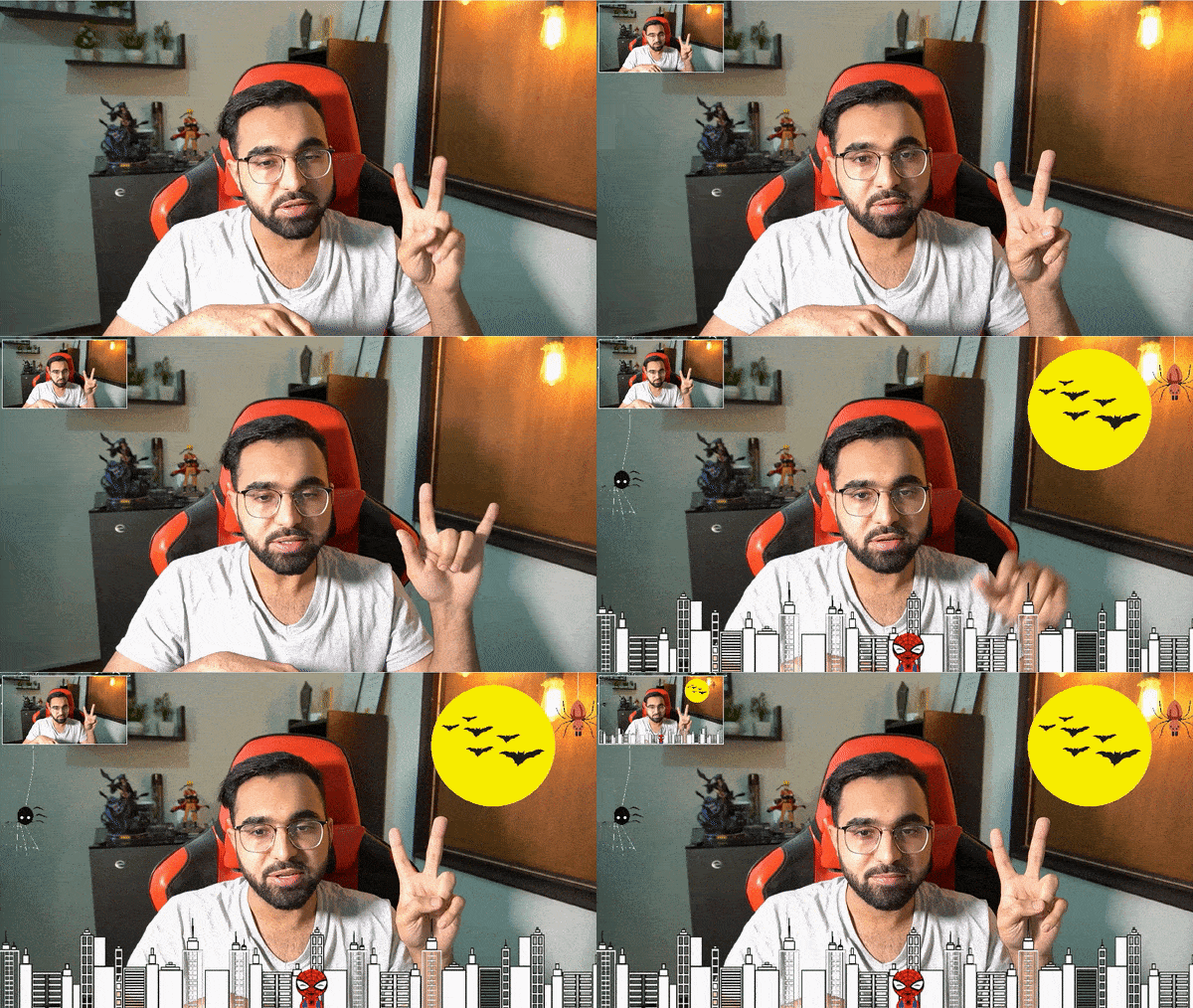
In this week’s tutorial, we’ll learn to utilize the landmarks to count and fingers (that are up) in images and videos and create a real-time hand counter. We will also create a hand finger recognition and visualization application that will display the exact fingers that are up. This will work for both hands.
Then based on the status (i.e., up/down) of the fingers, we will build a Hand Gesture Recognizer that will be capable of identifying multiple gestures.
Below are the results on a few sample images but this will also work on camera feed in real-time and on recorded videos as well.
You will not need any expensive GPU, your CPU will suffice as the whole code is highly optimized.
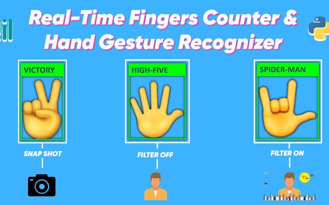
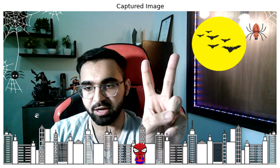
And that is not all, in the end, on top of all this, we will build a Selfie-Capturing System that will be controlled using hand gestures to enhance the user experience. So we will be able to capture images and also turn an image filter on/off without even touching our device. The image below shows a visual of what this system will be capable of.
Well 🤔, maybe not exactly that but somewhat similar.
Excited yet? I know I am! Before diving into the implementation, let me tell you that as a child, I always was fascinated with the concept of automating the interaction between people and machines and that was one of the reasons I got into programming.
To be more precise, I wanted to control my computer with my mind, yes I know how this sounds but I was just a kid back then. Controlling computers via mind with high fidelity is not feasible yet but hey Elon, is working on it.. So there’s still hope.
But for now, why don’t we utilize the options we have. I have published some other tutorials too on controlling different applications using hand body gestures.
So I can tell you that using hand gestures to interact with a system is a much better option than using some other part like the mouth since hands are capable of making multiple shapes and gestures without much effort.
Also during these crucial times of covid-19, it is very unsafe to touch the devices installed at public places like ATMs. So upgrading these to make them operable via gestures can tremendously reduce infection risk..
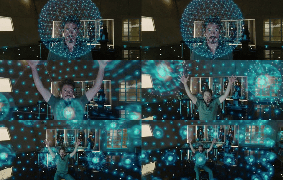
Tony Stark, the boy Genius can be seen in movies to control stuff with his hand gestures, so why let him have all the fun when we can join the party too.
You can also use the techniques you’ll learn in this tutorial to control any other Human-Computer Interaction based application.
The tutorial is divided into small steps with every step explained in detail in the simplest manner possible.
Alright, so without further ado, let’s get started.
Import the Libraries
First, we will import the required libraries.
import cv2
import time
import pygame
import numpy as np
import mediapipe as mp
import matplotlib.pyplot as plt
Initialize the Hands Landmarks Detection Model
After that, we will need to initialize the mp.solutions.hands class and then set up the mp.solutions.hands.Hands() function with appropriate arguments and also initialize mp.solutions.drawing_utils class that is required to visualize the detected landmarks. We will be working with images and videos as well, so we will have to set up the mp.solutions.hands.Hands() function two times.
Once with the argument static_image_mode set to True to use with images and the second time static_image_mode set to False to use with videos. This speeds up the landmarks detection process, and the intuition behind this was explained in detail in the previous post.
# Initialize the mediapipe hands class.
mp_hands = mp.solutions.hands

# Set up the Hands functions for images and videos.
hands = mp_hands.Hands(static_image_mode=True, max_num_hands=2, min_detection_confidence=0.5)
hands_videos = mp_hands.Hands(static_image_mode=False, max_num_hands=2, min_detection_confidence=0.5)

# Initialize the mediapipe drawing class.
mp_drawing = mp.solutions.drawing_utils
Step 1: Perform Hands Landmarks Detection
In the step, we will create a function detectHandsLandmarks() that will take an image/frame as input and will perform the landmarks detection on the hands in the image/frame using the solution provided by Mediapipe and will get twenty-one 3D landmarks for each hand in the image. The function will display or return the results depending upon the passed arguments.
The function is quite similar to the one in the previous post, so if you had read the post, you can skip this step. I could have imported it from a separate .py file, but I didn’t, as I wanted to make this tutorial with the minimal number of prerequisites possible.
def detectHandsLandmarks(image, hands, draw=True, display = True):
    '''
    This function performs hands landmarks detection on an image.
    Args:
        image:   The input image with prominent hand(s) whose landmarks needs to be detected.
        hands:   The Hands function required to perform the hands landmarks detection.
        draw:    A boolean value that is if set to true the function draws hands landmarks on the output image.
        display: A boolean value that is if set to true the function displays the original input image, and the output
                 image with hands landmarks drawn if it was specified and returns nothing.
    Returns:
        output_image: A copy of input image with the detected hands landmarks drawn if it was specified.
        results:      The output of the hands landmarks detection on the input image.
    '''

    # Create a copy of the input image to draw landmarks on.
    output_image = image.copy()

    # Convert the image from BGR into RGB format.
    imgRGB = cv2.cvtColor(image, cv2.COLOR_BGR2RGB)

    # Perform the Hands Landmarks Detection.
    results = hands.process(imgRGB)

    # Check if landmarks are found and are specified to be drawn.
    if results.multi_hand_landmarks and draw:

        # Iterate over the found hands.
        for hand_landmarks in results.multi_hand_landmarks:

            # Draw the hand landmarks on the copy of the input image.
            mp_drawing.draw_landmarks(image = output_image, landmark_list = hand_landmarks,
                                      connections = mp_hands.HAND_CONNECTIONS,
                                      landmark_drawing_spec=mp_drawing.DrawingSpec(color=(255,255,255),
                                                                                   thickness=2, circle_radius=2),
                                      connection_drawing_spec=mp_drawing.DrawingSpec(color=(0,255,0),
                                                                                     thickness=2, circle_radius=2))

    # Check if the original input image and the output image are specified to be displayed.
    if display:

        # Display the original input image and the output image.
        plt.figure(figsize=[15,15])
        plt.subplot(121);plt.imshow(image[:,:,::-1]);plt.title("Original Image");plt.axis('off');
        plt.subplot(122);plt.imshow(output_image[:,:,::-1]);plt.title("Output");plt.axis('off');

    # Otherwise
    else:

        # Return the output image and results of hands landmarks detection.
        return output_image, results
Now let’s test the function detectHandsLandmarks() created above to perform hands landmarks detection on a sample image and display the results.
# Read a sample image and perform hands landmarks detection on it.
image = cv2.imread('media/sample.jpg')
detectHandsLandmarks(image, hands, display=True)
Great! got the required landmarks so the function is working accurately.
Step 2: Build the Fingers Counter
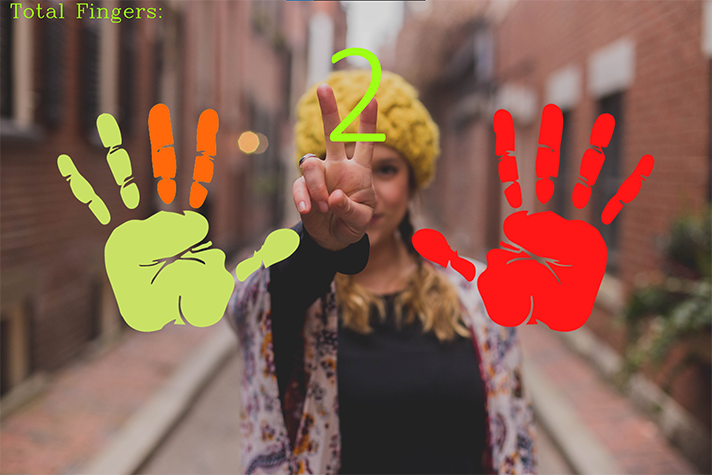
Now in this step, we will create a function countFingers() that will take in the results of the landmarks detection returned by the function detectHandsLandmarks() and will utilize the landmarks to count the number of fingers up of each hand in the image/frame and will return the count and the status of each finger in the image as well.
How will it work?
To check the status of each finger (i.e., either it is up or not), we will compare the y-coordinates of the FINGER_TIP landmark and FINGER_PIP landmark of each finger. Whenever the finger will be up, the y-coordinate of the FINGER_TIP landmark will have a lower value than the FINGER_PIP landmark.
But for the thumbs, the scenario will be a little different as we will have to compare the x-coordinates of the THUMB_TIP landmark and THUMB_MCP landmark and the condition will vary depending upon whether the hand is left or right.
For the right hand, whenever the thumb will be open, the x-coordinate of the THUMB_TIP landmark will have a lower value than the THUMB_MCP landmark, and for the left hand, the x-coordinate of the THUMB_TIP landmark will have a greater value than the THUMB_MCP landmark.
Note:You have to face the palm of your hand towards the camera.
def countFingers(image, results, draw=True, display=True):
    '''
    This function will count the number of fingers up for each hand in the image.
    Args:
        image:   The image of the hands on which the fingers counting is required to be performed.
        results: The output of the hands landmarks detection performed on the image of the hands.
        draw:    A boolean value that is if set to true the function writes the total count of fingers of the hands on the
                 output image.
        display: A boolean value that is if set to true the function displays the resultant image and returns nothing.
    Returns:
        output_image:     A copy of the input image with the fingers count written, if it was specified.
        fingers_statuses: A dictionary containing the status (i.e., open or close) of each finger of both hands.
        count:            A dictionary containing the count of the fingers that are up, of both hands.
    '''

    # Get the height and width of the input image.
    height, width, _ = image.shape

    # Create a copy of the input image to write the count of fingers on.
    output_image = image.copy()

    # Initialize a dictionary to store the count of fingers of both hands.
    count = {'RIGHT': 0, 'LEFT': 0}

    # Store the indexes of the tips landmarks of each finger of a hand in a list.
    fingers_tips_ids = [mp_hands.HandLandmark.INDEX_FINGER_TIP, mp_hands.HandLandmark.MIDDLE_FINGER_TIP,
                        mp_hands.HandLandmark.RING_FINGER_TIP, mp_hands.HandLandmark.PINKY_TIP]

    # Initialize a dictionary to store the status (i.e., True for open and False for close) of each finger of both hands.
    fingers_statuses = {'RIGHT_THUMB': False, 'RIGHT_INDEX': False, 'RIGHT_MIDDLE': False, 'RIGHT_RING': False,
                        'RIGHT_PINKY': False, 'LEFT_THUMB': False, 'LEFT_INDEX': False, 'LEFT_MIDDLE': False,
                        'LEFT_RING': False, 'LEFT_PINKY': False}


    # Iterate over the found hands in the image.
    for hand_index, hand_info in enumerate(results.multi_handedness):

        # Retrieve the label of the found hand.
        hand_label = hand_info.classification[0].label

        # Retrieve the landmarks of the found hand.
        hand_landmarks =  results.multi_hand_landmarks[hand_index]

        # Iterate over the indexes of the tips landmarks of each finger of the hand.
        for tip_index in fingers_tips_ids:

            # Retrieve the label (i.e., index, middle, etc.) of the finger on which we are iterating upon.
            finger_name = tip_index.name.split("_")[0]

            # Check if the finger is up by comparing the y-coordinates of the tip and pip landmarks.
            if (hand_landmarks.landmark[tip_index].y < hand_landmarks.landmark[tip_index - 2].y):

                # Update the status of the finger in the dictionary to true.
                fingers_statuses[hand_label.upper()+"_"+finger_name] = True

                # Increment the count of the fingers up of the hand by 1.
                count[hand_label.upper()] += 1

        # Retrieve the y-coordinates of the tip and mcp landmarks of the thumb of the hand.
        thumb_tip_x = hand_landmarks.landmark[mp_hands.HandLandmark.THUMB_TIP].x
        thumb_mcp_x = hand_landmarks.landmark[mp_hands.HandLandmark.THUMB_TIP - 2].x

        # Check if the thumb is up by comparing the hand label and the x-coordinates of the retrieved landmarks.
        if (hand_label=='Right' and (thumb_tip_x < thumb_mcp_x)) or (hand_label=='Left' and (thumb_tip_x > thumb_mcp_x)):

            # Update the status of the thumb in the dictionary to true.
            fingers_statuses[hand_label.upper()+"_THUMB"] = True

            # Increment the count of the fingers up of the hand by 1.
            count[hand_label.upper()] += 1

    # Check if the total count of the fingers of both hands are specified to be written on the output image.
    if draw:

        # Write the total count of the fingers of both hands on the output image.
        cv2.putText(output_image, " Total Fingers: ", (10, 25),cv2.FONT_HERSHEY_COMPLEX, 1, (20,255,155), 2)
        cv2.putText(output_image, str(sum(count.values())), (width//2-150,240), cv2.FONT_HERSHEY_SIMPLEX,
                    8.9, (20,255,155), 10, 10)

    # Check if the output image is specified to be displayed.
    if display:

        # Display the output image.
        plt.figure(figsize=[10,10])
        plt.imshow(output_image[:,:,::-1]);plt.title("Output Image");plt.axis('off');

    # Otherwise
    else:

        # Return the output image, the status of each finger and the count of the fingers up of both hands.
        return output_image, fingers_statuses, count
Now we will utilize the function countFingers() created above on a real-time webcam feed to count the number of fingers in the frame.
# Initialize the VideoCapture object to read from the webcam.
camera_video = cv2.VideoCapture(1)
camera_video.set(3,1280)
camera_video.set(4,960)

# Create named window for resizing purposes.
cv2.namedWindow('Fingers Counter', cv2.WINDOW_NORMAL)

# Iterate until the webcam is accessed successfully.
while camera_video.isOpened():

    # Read a frame.
    ok, frame = camera_video.read()

    # Check if frame is not read properly then continue to the next iteration to read the next frame.
    if not ok:
        continue

    # Flip the frame horizontally for natural (selfie-view) visualization.
    frame = cv2.flip(frame, 1)

    # Perform Hands landmarks detection on the frame.
    frame, results = detectHandsLandmarks(frame, hands_videos, display=False)

    # Check if the hands landmarks in the frame are detected.
    if results.multi_hand_landmarks:

        # Count the number of fingers up of each hand in the frame.
        frame, fingers_statuses, count = countFingers(frame, results, display=False)

    # Display the frame.
    cv2.imshow('Fingers Counter', frame)

    # Wait for 1ms. If a key is pressed, retreive the ASCII code of the key.
    k = cv2.waitKey(1) & 0xFF

    # Check if 'ESC' is pressed and break the loop.
    if(k == 27):
        break

# Release the VideoCapture Object and close the windows.
camera_video.release()
cv2.destroyAllWindows()
Output Video
Astonishing! the fingers are being counted very fast.
Step 3: Visualize the Counted Fingers
Now that we have built the finger counter, in this step, we will visualize the status (up or down) of each finger in the image/frame in a very appealing way. We will draw left and right handprints on the image and will change the color of the handprints in real-time depending upon the output (i.e., status (up or down) of each finger) from the function countFingers().
The hand print will be Red if that particular hand (i.e., either right or left) is not present in the image/frame.
The hand print will be Green if the hand is present in the image/frame.
The fingers of the hand print, that are up, will be highlighted by with the Orange color and the fingers that are down, will remain Green.
To accomplish this, we will create a function annotate() that will take in the output of the function countFingers() and will utilize it to simply overlay the required hands and fingers prints on the image/frame in the required color.
We have the .png images of the hands and fingers prints in the required colors (red, green, and orange) with transparent backgrounds, so we will only need to select the appropriate images depending upon the hands and fingers statuses and overlay them on the image/frame. You will also get these images with the code when you will download them.
def annotate(image, results, fingers_statuses, count, display=True):
    '''
    This function will draw an appealing visualization of each fingers up of the both hands in the image.
    Args:
        image:            The image of the hands on which the counted fingers are required to be visualized.
        results:          The output of the hands landmarks detection performed on the image of the hands.
        fingers_statuses: A dictionary containing the status (i.e., open or close) of each finger of both hands.
        count:            A dictionary containing the count of the fingers that are up, of both hands.
        display:          A boolean value that is if set to true the function displays the resultant image and
                          returns nothing.
    Returns:
        output_image: A copy of the input image with the visualization of counted fingers.
    '''

    # Get the height and width of the input image.
    height, width, _ = image.shape

    # Create a copy of the input image.
    output_image = image.copy()

    # Select the images of the hands prints that are required to be overlayed.
    ########################################################################################################################

    # Initialize a dictionaty to store the images paths of the both hands.
    # Initially it contains red hands images paths. The red image represents that the hand is not present in the image.
    HANDS_IMGS_PATHS = {'LEFT': ['media/left_hand_not_detected.png'], 'RIGHT': ['media/right_hand_not_detected.png']}

    # Check if there is hand(s) in the image.
    if results.multi_hand_landmarks:

        # Iterate over the detected hands in the image.
        for hand_index, hand_info in enumerate(results.multi_handedness):

            # Retrieve the label of the hand.
            hand_label = hand_info.classification[0].label

            # Update the image path of the hand to a green color hand image.
            # This green image represents that the hand is present in the image.
            HANDS_IMGS_PATHS[hand_label.upper()] = ['media/'+hand_label.lower()+'_hand_detected.png']

            # Check if all the fingers of the hand are up/open.
            if count[hand_label.upper()] == 5:

                # Update the image path of the hand to a hand image with green color palm and orange color fingers image.
                # The orange color of a finger represents that the finger is up.
                HANDS_IMGS_PATHS[hand_label.upper()] = ['media/'+hand_label.lower()+'_all_fingers.png']

            # Otherwise if all the fingers of the hand are not up/open.
            else:

                # Iterate over the fingers statuses of the hands.
                for finger, status in fingers_statuses.items():

                    # Check if the finger is up and belongs to the hand that we are iterating upon.
                    if status == True and finger.split("_")[0] == hand_label.upper():

                        # Append another image of the hand in the list inside the dictionary.
                        # This image only contains the finger we are iterating upon of the hand in orange color.
                        # As the orange color represents that the finger is up.
                        HANDS_IMGS_PATHS[hand_label.upper()].append('media/'+finger.lower()+'.png')

    ########################################################################################################################

    # Overlay the selected hands prints on the input image.
    ########################################################################################################################

    # Iterate over the left and right hand.
    for hand_index, hand_imgs_paths in enumerate(HANDS_IMGS_PATHS.values()):

        # Iterate over the images paths of the hand.
        for img_path in hand_imgs_paths:

            # Read the image including its alpha channel. The alpha channel (0-255) determine the level of visibility.
            # In alpha channel, 0 represents the transparent area and 255 represents the visible area.
            hand_imageBGRA = cv2.imread(img_path, cv2.IMREAD_UNCHANGED)

            # Retrieve all the alpha channel values of the hand image.
            alpha_channel = hand_imageBGRA[:,:,-1]

            # Retrieve all the blue, green, and red channels values of the hand image.
            # As we also need the three-channel version of the hand image.
            hand_imageBGR  = hand_imageBGRA[:,:,:-1]

            # Retrieve the height and width of the hand image.
            hand_height, hand_width, _ = hand_imageBGR.shape

            # Retrieve the region of interest of the output image where the handprint image will be placed.
            ROI = output_image[30 : 30 + hand_height,
                               (hand_index * width//2) + width//12 : ((hand_index * width//2) + width//12 + hand_width)]

            # Overlay the handprint image by updating the pixel values of the ROI of the output image at the
            # indexes where the alpha channel has the value 255.
            ROI[alpha_channel==255] = hand_imageBGR[alpha_channel==255]

            # Update the ROI of the output image with resultant image pixel values after overlaying the handprint.
            output_image[30 : 30 + hand_height,
                         (hand_index * width//2) + width//12 : ((hand_index * width//2) + width//12 + hand_width)] = ROI

    ########################################################################################################################

    # Check if the output image is specified to be displayed.
    if display:

        # Display the output image.
        plt.figure(figsize=[10,10])
        plt.imshow(output_image[:,:,::-1]);plt.title("Output Image");plt.axis('off');

    # Otherwise
    else:

        # Return the output image
        return output_image
Now we will use the function annotate() created above on a webcam feed in real-time to visualize the results of the fingers counter.
# Initialize the VideoCapture object to read from the webcam.
camera_video = cv2.VideoCapture(1)
camera_video.set(3,1280)
camera_video.set(4,960)

# Create named window for resizing purposes.
cv2.namedWindow('Counted Fingers Visualization', cv2.WINDOW_NORMAL)

# Iterate until the webcam is accessed successfully.
while camera_video.isOpened():

    # Read a frame.
    ok, frame = camera_video.read()

    # Check if frame is not read properly then continue to the next iteration to read the next frame.
    if not ok:
        continue

    # Flip the frame horizontally for natural (selfie-view) visualization.
    frame = cv2.flip(frame, 1)

    # Perform Hands landmarks detection on the frame.
    frame, results = detectHandsLandmarks(frame, hands_videos, display=False)

    # Check if the hands landmarks in the frame are detected.
    if results.multi_hand_landmarks:

        # Count the number of fingers up of each hand in the frame.
        frame, fingers_statuses, count = countFingers(frame, results, display=False)

    # Visualize the counted fingers.
    frame = annotate(frame, results, fingers_statuses, count, display=False)

    # Display the frame.
    cv2.imshow('Counted Fingers Visualization', frame)

    # Wait for 1ms. If a key is pressed, retreive the ASCII code of the key.
    k = cv2.waitKey(1) & 0xFF

    # Check if 'ESC' is pressed and break the loop.
    if(k == 27):
        break

# Release the VideoCapture Object and close the windows.
camera_video.release()
cv2.destroyAllWindows()
Output Video
Woah! that was Cool, the results are delightful.
Step 4: Build the Hand Gesture Recognizer
We will create a function recognizeGestures() in this step, that will use the status (i.e., up or down) of the fingers outputted by the function countFingers() to determine the gesture of the hands in the image. The function will be capable of identifying the following hand gestures:
V Hand Gesture ✌️ (i.e., only the index and middle finger up)
SPIDERMAN Hand Gesture 🤟 (i.e., the thumb, index, and pinky finger up)
HIGH-FIVE Hand Gesture ✋ (i.e., all the five fingers up)
For the sake of simplicity, we are only limiting this to three hand gestures. But if you want, you can easily extend this function to make it capable of identifying more gestures just by adding more conditional statements.
def recognizeGestures(image, fingers_statuses, count, draw=True, display=True):
    '''
    This function will determine the gesture of the left and right hand in the image.
    Args:
        image:            The image of the hands on which the hand gesture recognition is required to be performed.
        fingers_statuses: A dictionary containing the status (i.e., open or close) of each finger of both hands.
        count:            A dictionary containing the count of the fingers that are up, of both hands.
        draw:             A boolean value that is if set to true the function writes the gestures of the hands on the
                          output image, after recognition.
        display:          A boolean value that is if set to true the function displays the resultant image and
                          returns nothing.
    Returns:
        output_image:   A copy of the input image with the left and right hand recognized gestures written if it was
                        specified.
        hands_gestures: A dictionary containing the recognized gestures of the right and left hand.
    '''

    # Create a copy of the input image.
    output_image = image.copy()

    # Store the labels of both hands in a list.
    hands_labels = ['RIGHT', 'LEFT']

    # Initialize a dictionary to store the gestures of both hands in the image.
    hands_gestures = {'RIGHT': "UNKNOWN", 'LEFT': "UNKNOWN"}

    # Iterate over the left and right hand.
    for hand_index, hand_label in enumerate(hands_labels):

        # Initialize a variable to store the color we will use to write the hands gestures on the image.
        # Initially it is red which represents that the gesture is not recognized.
        color = (0, 0, 255)

        # Check if the person is making the 'V' gesture with the hand.
        ####################################################################################################################

        # Check if the number of fingers up is 2 and the fingers that are up, are the index and the middle finger.
        if count[hand_label] == 2  and fingers_statuses[hand_label+'_MIDDLE'] and fingers_statuses[hand_label+'_INDEX']:

            # Update the gesture value of the hand that we are iterating upon to V SIGN.
            hands_gestures[hand_label] = "V SIGN"

            # Update the color value to green.
            color=(0,255,0)

        ####################################################################################################################

        # Check if the person is making the 'SPIDERMAN' gesture with the hand.
        ##########################################################################################################################################################

        # Check if the number of fingers up is 3 and the fingers that are up, are the thumb, index and the pinky finger.
        elif count[hand_label] == 3 and fingers_statuses[hand_label+'_THUMB'] and fingers_statuses[hand_label+'_INDEX'] and fingers_statuses[hand_label+'_PINKY']:

            # Update the gesture value of the hand that we are iterating upon to SPIDERMAN SIGN.
            hands_gestures[hand_label] = "SPIDERMAN SIGN"

            # Update the color value to green.
            color=(0,255,0)

        ##########################################################################################################################################################

        # Check if the person is making the 'HIGH-FIVE' gesture with the hand.
        ####################################################################################################################

        # Check if the number of fingers up is 5, which means that all the fingers are up.
        elif count[hand_label] == 5:

            # Update the gesture value of the hand that we are iterating upon to HIGH-FIVE SIGN.
            hands_gestures[hand_label] = "HIGH-FIVE SIGN"

            # Update the color value to green.
            color=(0,255,0)

        ####################################################################################################################

        # Check if the hands gestures are specified to be written.
        if draw:

            # Write the hand gesture on the output image.
            cv2.putText(output_image, hand_label +': '+ hands_gestures[hand_label] , (10, (hand_index+1) * 60),
                        cv2.FONT_HERSHEY_PLAIN, 4, color, 5)


    # Check if the output image is specified to be displayed.
    if display:

        # Display the output image.
        plt.figure(figsize=[10,10])
        plt.imshow(output_image[:,:,::-1]);plt.title("Output Image");plt.axis('off');

    # Otherwise
    else:

        # Return the output image and the gestures of the both hands.
        return output_image, hands_gestures
Now we will utilize the function recognizeGestures() created above to perform hand gesture recognition on a few sample images and display the results.
# Read a sample image and perform the hand gesture recognition on it after flipping it horizontally.
image = cv2.imread('media/sample1.jpg')
flipped_image = cv2.flip(image, 1)
_, results = detectHandsLandmarks(flipped_image, hands, display=False)
if results.multi_hand_landmarks:
    output_image, fingers_statuses, count = countFingers(image, results, draw=False, display = False)
    recognizeGestures(image, fingers_statuses, count)
# Read another sample image and perform the hand gesture recognition on it after flipping it horizontally.
image = cv2.imread('media/sample2.jpg')
flipped_image = cv2.flip(image, 1)
_, results = detectHandsLandmarks(flipped_image, hands, display=False)
if results.multi_hand_landmarks:
    output_image, fingers_statuses, count =countFingers(image, results, draw=False, display = False)
# Read another sample image and perform the hand gesture recognition on it after flipping it horizontally.
image = cv2.imread('media/sample3.jpg')
flipped_image = cv2.flip(image, 1)
_, results = detectHandsLandmarks(flipped_image, hands, display=False)
if results.multi_hand_landmarks:
    output_image, fingers_statuses, count =countFingers(image, results, draw=False, display = False)
    recognizeGestures(image, fingers_statuses, count)
Step 5: Build a Selfie-Capturing System controlled by Hand Gestures
In the last step, we will utilize the gesture recognizer we had made in the last step to trigger a few events. As our gesture recognizer can identify only three gestures (i.e., V Hand Gesture (✌️), SPIDERMAN Hand Gesture (🤟), and HIGH-FIVE Hand Gesture (✋)).
So to get the most out of it, we will create a Selfie-Capturing System that will be controlled using hand gestures. We will allow the user to capture and store images into the disk using the ✌️ gesture. And to spice things up, we will also implement a filter applying mechanism in our system that will be controlled by the other two gestures. To apply the filter on the image/frame the 🤟 gesture will be used and the ✋ gesture will be used to turn off the filter.
# Initialize the VideoCapture object to read from the webcam.
camera_video = cv2.VideoCapture(1)
camera_video.set(3,1280)
camera_video.set(4,960)

# Create named window for resizing purposes.
cv2.namedWindow('Selfie-Capturing System', cv2.WINDOW_NORMAL)

# Read the filter image with its blue, green, red, and alpha channel.
filter_imageBGRA = cv2.imread('media/filter.png', cv2.IMREAD_UNCHANGED)

# Initialize a variable to store the status of the filter (i.e., whether to apply the filter or not).
filter_on = False

# Initialize the pygame modules and load the image-capture music file.
pygame.init()
pygame.mixer.music.load("media/cam.mp3")

# Initialize the number of consecutive frames on which we want to check the hand gestures before triggering the events.
num_of_frames = 5

# Initialize a dictionary to store the counts of the consecutive frames with the hand gestures recognized.
counter = {'V SIGN': 0, 'SPIDERMAN SIGN': 0, 'HIGH-FIVE SIGN': 0}

# Initialize a variable to store the captured image.
captured_image = None

# Iterate until the webcam is accessed successfully.
while camera_video.isOpened():

    # Read a frame.
    ok, frame = camera_video.read()

    # Check if frame is not read properly then continue to the next iteration to read the next frame.
    if not ok:
        continue

    # Flip the frame horizontally for natural (selfie-view) visualization.
    frame = cv2.flip(frame, 1)

    # Get the height and width of the frame of the webcam video.
    frame_height, frame_width, _ = frame.shape

    # Resize the filter image to the size of the frame.
    filter_imageBGRA = cv2.resize(filter_imageBGRA, (frame_width, frame_height))

    # Get the three-channel (BGR) image version of the filter image.
    filter_imageBGR  = filter_imageBGRA[:,:,:-1]

    # Perform Hands landmarks detection on the frame.
    frame, results = detectHandsLandmarks(frame, hands_videos, draw=False, display=False)

    # Check if the hands landmarks in the frame are detected.
    if results.multi_hand_landmarks:

        # Count the number of fingers up of each hand in the frame.
        frame, fingers_statuses, count = countFingers(frame, results, draw=False, display=False)

        # Perform the hand gesture recognition on the hands in the frame.
        _, hands_gestures = recognizeGestures(frame, fingers_statuses, count, draw=False, display=False)

        # Apply and Remove Image Filter Functionality.
        ####################################################################################################################

        # Check if any hand is making the SPIDERMAN hand gesture in the required number of consecutive frames.
        ####################################################################################################################

        # Check if the gesture of any hand in the frame is SPIDERMAN SIGN.
        if any(hand_gesture == "SPIDERMAN SIGN" for hand_gesture in hands_gestures.values()):

            # Increment the count of consecutive frames with SPIDERMAN hand gesture recognized.
            counter['SPIDERMAN SIGN'] += 1

            # Check if the counter is equal to the required number of consecutive frames.
            if counter['SPIDERMAN SIGN'] == num_of_frames:

                # Turn on the filter by updating the value of the filter status variable to true.
                filter_on = True

                # Update the counter value to zero.
                counter['SPIDERMAN SIGN'] = 0

        # Otherwise if the gesture of any hand in the frame is not SPIDERMAN SIGN.
        else:

            # Update the counter value to zero. As we are counting the consective frames with SPIDERMAN hand gesture.
            counter['SPIDERMAN SIGN'] = 0

        ####################################################################################################################

        # Check if any hand is making the HIGH-FIVE hand gesture in the required number of consecutive frames.
        ####################################################################################################################

        # Check if the gesture of any hand in the frame is HIGH-FIVE SIGN.
        if any(hand_gesture == "HIGH-FIVE SIGN" for hand_gesture in hands_gestures.values()):

            # Increment the count of consecutive frames with HIGH-FIVE hand gesture recognized.
            counter['HIGH-FIVE SIGN'] += 1

            # Check if the counter is equal to the required number of consecutive frames.
            if counter['HIGH-FIVE SIGN'] == num_of_frames:

                # Turn off the filter by updating the value of the filter status variable to False.
                filter_on = False

                # Update the counter value to zero.
                counter['HIGH-FIVE SIGN'] = 0

        # Otherwise if the gesture of any hand in the frame is not HIGH-FIVE SIGN.
        else:

            # Update the counter value to zero. As we are counting the consective frames with HIGH-FIVE hand gesture.
            counter['HIGH-FIVE SIGN'] = 0

        ####################################################################################################################

    # Check if the filter is turned on.
    if filter_on:

        # Apply the filter by updating the pixel values of the frame at the indexes where the
        # alpha channel of the filter image has the value 255.
        frame[filter_imageBGRA[:,:,-1]==255] = filter_imageBGR[filter_imageBGRA[:,:,-1]==255]

        ####################################################################################################################

    # Image Capture Functionality.
    ########################################################################################################################

    # Check if the hands landmarks are detected and the gesture of any hand in the frame is V SIGN.
    if results.multi_hand_landmarks and any(hand_gesture == "V SIGN" for hand_gesture in hands_gestures.values()):

        # Increment the count of consecutive frames with V hand gesture recognized.
        counter['V SIGN'] += 1

        # Check if the counter is equal to the required number of consecutive frames.
        if counter['V SIGN'] == num_of_frames:

            # Make a border around a copy of the current frame.
            captured_image = cv2.copyMakeBorder(src=frame, top=10, bottom=10, left=10, right=10,
                                                borderType=cv2.BORDER_CONSTANT, value=(255,255,255))

            # Capture an image and store it in the disk.
            cv2.imwrite('Captured_Image.png', captured_image)

            # Display a black image.
            cv2.imshow('Selfie-Capturing System', np.zeros((frame_height, frame_width)))

            # Play the image capture music to indicate the an image is captured and wait for 100 milliseconds.
            pygame.mixer.music.play()
            cv2.waitKey(100)

            # Display the captured image.
            plt.close();plt.figure(figsize=[10,10])
            plt.imshow(frame[:,:,::-1]);plt.title("Captured Image");plt.axis('off');

            # Update the counter value to zero.
            counter['V SIGN'] = 0

    # Otherwise if the gesture of any hand in the frame is not V SIGN.
    else:

        # Update the counter value to zero. As we are counting the consective frames with V hand gesture.
        counter['V SIGN'] = 0

    ########################################################################################################################

    # Check if we have captured an image.
    if captured_image is not None:

        # Resize the image to the 1/5th of its current width while keeping the aspect ratio constant.
        captured_image = cv2.resize(captured_image, (frame_width//5, int(((frame_width//5) / frame_width) * frame_height)))

        # Get the new height and width of the image.
        img_height, img_width, _ = captured_image.shape

        # Overlay the resized captured image over the frame by updating its pixel values in the region of interest.
        frame[10: 10+img_height, 10: 10+img_width] = captured_image

    # Display the frame.
    cv2.imshow('Selfie-Capturing System', frame)

    # Wait for 1ms. If a key is pressed, retreive the ASCII code of the key.
    k = cv2.waitKey(1) & 0xFF

    # Check if 'ESC' is pressed and break the loop.
    if(k == 27):
        break

# Release the VideoCapture Object and close the windows.
camera_video.release()
cv2.destroyAllWindows()
Output Video
As expected, the results are amazing, the system is working very smoothly. If you want, you can extend this system to have multiple filters and introduce another gesture to switch between the filters.
Join My Course Computer Vision For Building Cutting Edge Applications Course
The only course out there that goes beyond basic AI Applications and teaches you how to create next-level apps that utilize physics, deep learning, classical image processing, hand and body gestures. Don’t miss your chance to level up and take your career to new heights
You’ll Learn about:
Creating GUI interfaces for python AI scripts.
Creating .exe DL applications
Using a Physics library in Python & integrating it with AI
Advance Image Processing Skills
Advance Gesture Recognition with Mediapipe
Task Automation with AI & CV
Training an SVM machine Learning Model.
Creating & Cleaning an ML dataset from scratch.
Training DL models & how to use CNN’s & LSTMS.
Creating 10 Advance AI/CV Applications
& More
Whether you’re a seasoned AI professional or someone just looking to start out in AI, this is the course that will teach you, how to Architect & Build complex, real world and thrilling AI applications
In this tutorial, we have learned to perform landmarks detection on the prominent hands in images/videos, to get twenty-one 3D landmarks, and then use those landmarks to extract useful info about each finger of the hands i.e., whether the fingers are up or down. Using this methodology, we have created a finger counter and recognition system and then learned to visualize its results.
We have also built a hand gesture recognizer capable of identifying three different gestures of the hands in the images/videos based on the status (i.e., up or down) of the fingers in real-time and had utilized the recognizer in our Selfie-Capturing System to trigger multiple events.
Now here are a few limitations in our application that you should know about, for our finger counter to work properly the user has to face the palm of his hand towards the camera in front of him. As the directions of the thumbs change based upon the orientation of the hand. And the approach we are using completely depends upon the direction. See the image below.
But you can easily overcome this limitation by using accumulated angles of joints to check whether each finger is bent or straight. And for that, you can check out the tutorial I had published on Real-Time 3D Pose Detection as I had used a similar approach in it to classify the poses.
Another limitation is that we are using the finger counter to determine the gestures of the hands and unfortunately complex hand gestures can have the same fingers up/down like the victory hand gesture (✌), and crossed fingers gesture (🤞). To get around this, you can train a deep learning model on top of some target gestures.
You can reach out to me personally for a 1 on 1 consultation session in AI/computer vision regarding your project. Our talented team of vision engineers will help you every step of the way. Get on a call with me directlyhere.
Ready to seriously dive into State of the Art AI & Computer Vision? Then Sign up for these premium Courses by Bleed AI
In this post, you’ll learn in-depth about the five of the most easiest and effective face detection options available in python, along with the pros and cons of each one of them. You will become capable of obtaining the required balance in accuracy, speed, and efficiency in any given scenario.
The face detection methods we will be covering are:
Face Detection is one of the most common and simplest vision techniques out there, as the name implies, it detects (i.e., locates) the faces in the images and is the first and essential step for almost every face application like Face Recognition, Facial Landmarks Detection, Face Gesture Recognition, and Augmented Reality (AR) Filters, etc.
Other than these, one of its most common applications, that you must have used, is your mobile camera which detects your face and adjusts the camera focus automatically in real-time.
Also, for what it’s worth Tony Stark’s EDITH (Even Dead I’m The Hero) glasses, inherited by Peter Parker in the Spider-Man Far From Home movie, also uses Face Detection as an initial step to perform its functionalities. Cool 😊 … right?
Yeah I know .. I know, I needed to add a marvel reference into it, the whole post get’s cooler.
Face detection also serves as a ground for a lot of exciting face applications for e.g. You can even appoint Mr. Beans as the President 😂 using Deepfake.
But for now, let’s just go back to Face Detection.
The idea behind face detection is to make the computer capable of identifying what human face exactly is and detecting the features that are associated with the faces in images/videos which might not always be easy because of changing facial expression, orientation, lighting conditions, and occlusions due to face masks, glasses, etc.
But with enough training data covering all the possible scenarios, you can create a very robust face detector.
And people throughout the years have done just that, they have designed various algorithms for facial detection and in this post, we’ll explore 5 such algorithms.
As this is the most common and widely used technique, there are a lot of face detectors out there.
But which Algorithm is the best?
If you’re looking for a single solution then it’s a hard answer as each of the algorithms that we’re going to cover has its own pros and cons, take a look at the demos at the end for some comparison, and make sure to read the summary for the final verdict.
Alright, so without further ado, let’s dive in.
[optin-monster slug=”rhkojx1lcwd45akbz8u8″]
Import the Libraries
We will first import the required libraries.
import os
import cv2
import dlib
from time import time
import mediapipe as mp
import matplotlib.pyplot as plt
Algorithm 1: OpenCV Haar Cascade Face Detection
This face detector was introduced in 2001 and remained the state-of-the-art face detection algorithm for many years. Other than just this face detector, OpenCV provides some other detectors (like eye, and smile, etc) too, which use the same haar cascade technique.
Load the OpenCV Haar Cascade Face Detector
To perform the face detection using this algorithm, first, we will have to load the pre-trained Haar cascade face detection model around 900 KBs from the disk, stored in a .xml file format, using the function CascadeClassifier().
# Load the pre-trained Haar cascade face detection model.
cascade_face_detector = cv2.CascadeClassifier("models/haarcascade_frontalface_default.xml")
cascade_face_detector
Create a Haar Cascade Face Detection Function
Now we will create a function haarCascadeDetectFaces() that will perform haar cascade face detection using the function cv2.CascadeClassifier.detectMultiScale() on an image/frame and will visualize the resultant image along with the original image (when working with images) or return the resultant image along with the output of the model (when working with videos) depending upon the passed arguments.
image – It is the input grayscale image containing the faces.
scaleFactor (optional) – It is the image size that is reduced at each image scale. Its default value is 1.1 which means a decrease of 10%.
minNeighbors (optional) – It is the number of minimum neighbors each predicted face should have, to retain. Otherwise, the prediction is ignored. Its default value is 3.
minSize (optional) – It is the minimum possible face size, the faces smaller than that size are ignored.
maxSize (optional) – It is the maximum possible face size, the faces larger than that are ignored. If maxSize == minSize then only the faces of a particular size are detected.
Returns:
results – It is an array of bounding boxes coordinates (i.e., x1, y1, bbox_width, bbox_height) where each bounding box encloses the detected face, the boxes may be partially outside the original image.
Note:When the value of the minNeighbors parameter is decreased, false positives are increased, and when the value of scaleFactor is decreased the large faces in the image become smaller and detectable by the algorithm at the cost of speed.
So the algorithm can detection very large and very small faces too by appropriately utilizing the scaleFactor argument.
def haarCascadeDetectFaces(image, cascade_face_detector, display = True):
    '''
    This function performs face(s) detection on an image using opencv haar cascade face detector.
    Args:
        image:                 The input image of the person(s) whose face needs to be detected.
        cascade_face_detector: The pre-trained Haar cascade face detection model loaded from the disk required to
                               perform the detection.
        display:               A boolean value that is if set to true the function displays the original input image,
                               and the output image with the bounding boxes drawn and time taken written and returns
                               nothing.
    Returns:
        output_image: A copy of input image with the bounding boxes drawn.
        results:      The output of the face detection process on the input image.
    '''

    # Get the height and width of the input image.
    image_height, image_width, _ = image.shape

    # Create a copy of the input image to draw bounding boxes on.
    output_image = image.copy()

    # Convert the input image to grayscale.
    gray = cv2.cvtColor(image, cv2.COLOR_BGR2GRAY)

    # Get the current time before performing face detection.
    start = time()

    # Perform the face detection on the image.
    results = cascade_face_detector.detectMultiScale(image=gray, scaleFactor=1.2, minNeighbors=3)

    # Get the current time after performing face detection.
    end = time()

    # Loop through each face detected in the image and retireve the bounding box cordinates.
    for (x1, y1, bbox_width, bbox_height) in results:

        # Draw bounding box around the face on the copy of the input image using the retrieved coordinates.
        cv2.rectangle(output_image, pt1=(x1, y1), pt2=(x1 + bbox_width, y1 + bbox_height), color=(0, 255, 0),
                      thickness=image_width//200)

    # Check if the original input image and the output image are specified to be displayed.
    if display:

        # Write the time take by face detection process on the output image.
        cv2.putText(output_image, text='Time taken: '+str(round(end - start, 2))+' Seconds.', org=(10, 65),
                    fontFace=cv2.FONT_HERSHEY_COMPLEX, fontScale=image_width//700, color=(0,0,255),
                    thickness=image_width//500)

        # Display the original input image and the output image.
        plt.figure(figsize=[15,15])
        plt.subplot(121);plt.imshow(image[:,:,::-1]);plt.title("Original Image");plt.axis('off');
        plt.subplot(122);plt.imshow(output_image[:,:,::-1]);plt.title("Output");plt.axis('off');

    # Otherwise
    else:

        # Return the output image and results of face detection.
        return output_image, results
Now we will utilize the function haarCascadeDetectFaces() created above to perform face detection on a few sample images and display the results.
# Read a sample image and perform haar cascade face detection on it.
image = cv2.imread('media/sample4.jpg')
haarCascadeDetectFaces(image, cascade_face_detector, display=True)
The time taken by the algorithm to perform detection is pretty impressive, so yeah, it can work in real-time on a CPU.
# Read another sample image and perform haar cascade face detection on it.
image = cv2.imread('media/sample5.jpg')
haarCascadeDetectFaces(image, cascade_face_detector, display=True)
A major drawback of this algorithm is that it does not work on non-frontal and occluded faces.
# Read another sample image and perform haar cascade face detection on it.
image = cv2.imread('media/sample1.jpg')
haarCascadeDetectFaces(image, cascade_face_detector, display=True)
And also gives a lot of false positives But that can be controlled by increasing the value of the minNeighbors argument in the function cv2.CascadeClassifier.detectMultiScale().
Algorithm 2: Dlib HoG Face Detection
This face detector is based on HoG (Histogram of Oriented Gradients), and SVM (Support Vector Machine) and is significantly more accurate than the previous one. The technique used in this one is not invariant to changes in face angle, so it uses five different HOG filters that are for:
Frontal face
Right side turned face
Left side turned face
Frontal face but rotated right
Frontal face but rotated left
So it can work on slightly non-frontal and rotated faces as well.
Load the Dlib HoG Face Detector
Now we will use the dlib.get_frontal_face_detector() function to load the pre-trained HoG face detector and we will not need to pass the path of the model file for this one as the model is included in the dlib library.
# Get the HoG face detection model.
hog_face_detector = dlib.get_frontal_face_detector()
hog_face_detector
Create a HoG Face Detection Function
Now we will create a function hogDetectFaces() that will perform HoG face detection by inputting the image/frame into the loaded hog_face_detector and will visualize the resultant image along with the original image or return the resultant image along with the output of HoG face detector depending upon the passed arguments.
Function Syntax:
results = hog_face_detector(image, upsample)
Parameters:
image – It is the input image containing the faces in RGB format.
upsample (optional) – It is the number of times to upsample an image before performing face detection.
Returns:
results – It is an array of rectangle objects containing the (x, y) coordinates of the corners of the bounding boxes enclosing the faces in the input image.
Note:The model is trained to detect a minimum face size of 80×80, so to detect small faces in the images, you will have to upsample the images that increase the resolution of the input images, thus increases the face size at the cost of computation speed of the detection process.
def hogDetectFaces(image, hog_face_detector, display = True):
    '''
    This function performs face(s) detection on an image using dlib hog face detector.
    Args:
        image:             The input image of the person(s) whose face needs to be detected.
        hog_face_detector: The hog face detection model required to perform the detection on the input image.
        display:           A boolean value that is if set to true the function displays the original input image,
                           and the output image with the bounding boxes drawn and time taken written and returns nothing.
    Returns:
        output_image: A copy of input image with the bounding boxes drawn.
        results:      The output of the face detection process on the input image.
    '''

    # Get the height and width of the input image.
    height, width, _ = image.shape

    # Create a copy of the input image to draw bounding boxes on.
    output_image = image.copy()

    # Convert the image from BGR into RGB format.
    imgRGB = cv2.cvtColor(image, cv2.COLOR_BGR2RGB)

    # Get the current time before performing face detection.
    start = time()

    # Perform the face detection on the image.
    results = hog_face_detector(imgRGB, 0)

    # Get the current time after performing face detection.
    end = time()

    # Loop through the bounding boxes of each face detected in the image.
    for bbox in results:

        # Retrieve the left most x-coordinate of the bounding box.
        x1 = bbox.left()

        # Retrieve the top most y-coordinate of the bounding box.
        y1 = bbox.top()

        # Retrieve the right most x-coordinate of the bounding box.
        x2 = bbox.right()

        # Retrieve the bottom most y-coordinate of the bounding box.
        y2 = bbox.bottom()

        # Draw a rectangle around a face on the copy of the image using the retrieved coordinates.
        cv2.rectangle(output_image, pt1=(x1, y1), pt2=(x2, y2), color=(0, 255, 0), thickness=width//200)


    # Check if the original input image and the output image are specified to be displayed.
    if display:

        # Write the time take by face detection process on the output image.
        cv2.putText(output_image, text='Time taken: '+str(round(end - start, 2))+' Seconds.', org=(10, 65),
                    fontFace=cv2.FONT_HERSHEY_COMPLEX, fontScale=width//700, color=(0,0,255), thickness=width//500)

        # Display the original input image and the output image.
        plt.figure(figsize=[15,15])
        plt.subplot(121);plt.imshow(image[:,:,::-1]);plt.title("Original Image");plt.axis('off');
        plt.subplot(122);plt.imshow(output_image[:,:,::-1]);plt.title("Output");plt.axis('off');

    # Otherwise
    else:

        # Return the output image and results of face detection.
        return output_image, results
Now we will utilize the function hogDetectFaces() created above to perform HoG face detection on a few sample images and display the results.
# Read a sample image and perform hog face detection on it.
image = cv2.imread('media/sample4.jpg')
hogDetectFaces(image, hog_face_detector, display=True)
So this too can work in real-time on a CPU. You can also resize the images before passing them to the model, as the smaller the images are, the faster the detection process will be. But this also increases the probability of faces smaller than 80×80 in the images.
# Read another sample image and perform hog face detection on it.
image = cv2.imread('media/sample3.jpg')
hogDetectFaces(image, hog_face_detector, display=True)
As you can see, it works on slightly rotated faces but will fail on extremely rotated and non-frontal ones and the bounding box often excludes some parts of the face like the chin and forehead.
# Read another sample image and perform hog face detection on it.
image = cv2.imread('media/sample7.jpg')
hogDetectFaces(image, hog_face_detector, display=True)
And also works on small occlusions but will fail on massive ones.
# Read another sample image and perform hog face detection on it.
image = cv2.imread('media/sample6.jpg')
hogDetectFaces(image, hog_face_detector, display=True)
As mentioned above, it cannot detect faces smaller than 80x80. Now, if you want, you can increase the upsample argument value of the loaded hog_face_detector in the function hogDetectFaces() created above, to detect the face in the image above, but that will also tremendously increase the time taken by the face detection process.
Algorithm 3: OpenCV Deep Learning based Face Detection
This one is based on a deep learning approach and uses ResNet-10 Architecture to detect multiple faces in a single pass (Single Shot Detector SSD) of the image through the network (model). It has been included in OpenCV since August 2017, with the official release of version 3.3, still, it is not as popular as the OpenCV Haar Cascade Face Detector but surely is highly more accurate.
Load the OpenCV Deep Learning based Face Detector
Now to load the face detector, OpenCV provides us with two options, one of them is in the Caffe framework’s format and takes around 5.10 MBs in memory and the other one is in the TensorFlow framework’s format and acquires only 2.7 MBs in memory.
To load the first one from the disk, we can use the cv2.dnn.readNetFromCaffe() function and to load the other one we will have to use the cv2.dnn.readNetFromTensorflow() function with appropriate arguments.
# Select the framework you want to use.
########################################################################################################################

# Load a model stored in Caffe framework's format using the architecture and the layers weights file stored in the disk.
opencv_dnn_model = cv2.dnn.readNetFromCaffe(prototxt="models/deploy.prototxt",
                                            caffeModel="models/res10_300x300_ssd_iter_140000_fp16.caffemodel")

########################################################## OR ##########################################################

# Load a model stored in TensorFlow framework's format using the architecture and the layers weights file stored in the disk
# opencv_dnn_model = cv2.dnn.readNetFromTensorflow(model="models/opencv_face_detector_uint8.pb",
#                                                  config="models/opencv_face_detector.pbtxt")

########################################################################################################################
opencv_dnn_model
Create an OpenCV Deep Learning based Face Detection Function
Now we will create a function cvDnnDetectFaces() that will perform Deep Learning-based face detection using OpenCV. First, we will pre-process the image/frame using the cv2.dnn.blobFromImage() function and then we will set the pre-processed image as an input to the network by using the function opencv_dnn_model.setInput().
And after that, pass the input image into the network by using the opencv_dnn_model.forward() function to get an array containing the bounding boxes coordinates normalized to ([0.0, 1.0]) and the detection confidence of each faces in the image.
After performing the detection, the function will also visualize the resultant image along with the original image or return the resultant image along with the output of the dnn face detector depending upon the passed arguments.
Note:Higher the face detection confidence score is, the more certain the model is about the detection.
def cvDnnDetectFaces(image, opencv_dnn_model, min_confidence=0.5, display = True):
    '''
    This function performs face(s) detection on an image using opencv deep learning based face detector.
    Args:
        image:               The input image of the person(s) whose face needs to be detected.
        opencv_dnn_model:    The pre-trained opencv deep learning based face detection model loaded from the disk
                             required to perform the detection.
        min_confidence:      The minimum detection confidence required to consider the face detection model's
                             prediction correct.
        display:             A boolean value that is if set to true the function displays the original input image,
                             and the output image with the bounding boxes drawn, confidence scores, and time taken
                             written and returns nothing.
    Returns:
        output_image: A copy of input image with the bounding boxes drawn and confidence scores written.
        results:      The output of the face detection process on the input image.
    '''

    # Get the height and width of the input image.
    image_height, image_width, _ = image.shape

    # Create a copy of the input image to draw bounding boxes and write confidence scores.
    output_image = image.copy()

    # Perform the required pre-processings on the image and create a 4D blob from image.
    # Resize the image and apply mean subtraction to its channels
    # Also convert from BGR to RGB format by swapping Blue and Red channels.
    preprocessed_image = cv2.dnn.blobFromImage(image, scalefactor=1.0, size=(300, 300),
                                               mean=(104.0, 117.0, 123.0), swapRB=False, crop=False)

    # Set the input value for the model.
    opencv_dnn_model.setInput(preprocessed_image)

    # Get the current time before performing face detection.
    start = time()

    # Perform the face detection on the image.
    results = opencv_dnn_model.forward()

    # Get the current time after performing face detection.
    end = time()

    # Loop through each face detected in the image.
    for face in results[0][0]:

        # Retrieve the face detection confidence score.
        face_confidence = face[2]

        # Check if the face detection confidence score is greater than the thresold.
        if face_confidence > min_confidence:

            # Retrieve the bounding box of the face.
            bbox = face[3:]

            # Retrieve the bounding box coordinates of the face and scale them according to the original size of the image.
            x1 = int(bbox[0] * image_width)
            y1 = int(bbox[1] * image_height)
            x2 = int(bbox[2] * image_width)
            y2 = int(bbox[3] * image_height)

            # Draw a bounding box around a face on the copy of the image using the retrieved coordinates.
            cv2.rectangle(output_image, pt1=(x1, y1), pt2=(x2, y2), color=(0, 255, 0), thickness=image_width//200)

            # Draw a filled rectangle near the bounding box of the face.
            # We are doing it to change the background of the confidence score to make it easily visible.
            cv2.rectangle(output_image, pt1=(x1, y1-image_width//20), pt2=(x1+image_width//16, y1),
                          color=(0, 255, 0), thickness=-1)

            # Write the confidence score of the face near the bounding box and on the filled rectangle.
            cv2.putText(output_image, text=str(round(face_confidence, 1)), org=(x1, y1-25),
                        fontFace=cv2.FONT_HERSHEY_COMPLEX, fontScale=image_width//700,
                        color=(255,255,255), thickness=image_width//200)

    # Check if the original input image and the output image are specified to be displayed.
    if display:

        # Write the time take by face detection process on the output image.
        cv2.putText(output_image, text='Time taken: '+str(round(end - start, 2))+' Seconds.', org=(10, 65),
                    fontFace=cv2.FONT_HERSHEY_COMPLEX, fontScale=image_width//700,
                    color=(0,0,255), thickness=image_width//500)

        # Display the original input image and the output image.
        plt.figure(figsize=[15,15])
        plt.subplot(121);plt.imshow(image[:,:,::-1]);plt.title("Original Image");plt.axis('off');
        plt.subplot(122);plt.imshow(output_image[:,:,::-1]);plt.title("Output");plt.axis('off');

    # Otherwise
    else:

        # Return the output image and results of face detection.
        return output_image, results
Now we will utilize the function cvDnnDetectFaces() created above to perform OpenCV deep learning-based face detection on a few sample images and display the results.
# Read a sample image and perform OpenCV dnn face detection on it.
image = cv2.imread('media/sample5.jpg')
cvDnnDetectFaces(image, opencv_dnn_model, display=True)
So it is highly more accurate than both of the above and works great even under massive occlusions and on non-frontal faces. And the reason for its significantly higher speed is that it can detect faces across various scales, allowing us to resize the images to a smaller size which decreases computations.
# Read another sample image and perform OpenCV dnn face detection on it.
image = cv2.imread('media/sample3.jpg')
cvDnnDetectFaces(image, opencv_dnn_model, display=True)
Also, the bounding box encloses the whole face, unlike the HoG Face Detector, making it easier to crop regions of interest (i.e., faces) from the images.CodeText
Also, the bounding box encloses the whole face, unlike the HoG Face Detector, making it easier to crop regions of interest (i.e., faces) from the images.CodeText
# Read another sample image and perform OpenCV dnn face detection on it.
image = cv2.imread('media/sample8.jpg')
cvDnnDetectFaces(image, opencv_dnn_model, display=True)
So even the faces with masks are detectable with this one.
Algorithm 4: Dlib Deep Learning based Face Detection
This detector is also based on a Deep learning (Convolution Neural Network) approach and uses Maximum-Margin Object Detection (MMOD) method to detect faces in images. This one is also trained for a minimum face size of 80×80 and provides the option of upsampling the images. This one is very slow on a CPU but can be used on an NVIDIA GPU and outperforms the other detectors in speed on the GPU.
Load the Dlib Deep Learning based Face Detector
Now first, we will use the dlib.cnn_face_detection_model_v1() function to load the pre-trained maximum-margin cnn face detector around 700 KBs from the disk, stored in a .dat file format.
# Load the dlib dnn face detection model from the file stored in the disk.
cnn_face_detector = dlib.cnn_face_detection_model_v1("models/mmod_human_face_detector.dat")
cnn_face_detector
Create a Dlib Deep Learning based Face Detection Function
Now we will create a function dlibDnnDetectFaces() in which we will perform deep Learning-based face detection using dlib by inputting the image/frame and the number of times to upsample the image to the loaded cnn_face_detector as we had done for the HoG face detection.
The only difference is that we are loading a different model, and it will return a list of objects, where each object will be a wrapper around a rectangle object (containing the bounding box coordinates) and a detection confidence score. As our every other function, this one will also visualize the results or return them depending upon the passed arguments.
def dlibDnnDetectFaces(image, cnn_face_detector, new_width = 600, display = True):
    '''
    This function performs face(s) detection on an image using dlib deep learning based face detector.
    Args:
        image:              The input image of the person(s) whose face needs to be detected.
        cnn_face_detector:  The pre-trained dlib deep learning based (CNN) face detection model loaded from
                            the disk required to perform the detection.
        new_width:          The new width of the input image to which it will be resized before passing it to the model.
        display:            A boolean value that is if set to true the function displays the original input image,
                            and the output image with the bounding boxes drawn, confidence scores, and time taken
                            written and returns nothing.
    Returns:
        output_image: A copy of input image with the bounding boxes drawn and confidence scores written.
        results:      The output of the face detection process on the input image.
    '''

    # Get the height and width of the input image.
    height, width, _ = image.shape

    # Calculate the new height of the input image while keeping the aspect ratio constant.
    new_height = int((new_width / width) * height)

    # Resize a copy of input image while keeping the aspect ratio constant.
    resized_image = cv2.resize(image.copy(), (new_width, new_height))

    # Convert the resized image from BGR into RGB format.
    imgRGB = cv2.cvtColor(resized_image, cv2.COLOR_BGR2RGB)

    # Create a copy of the input image to draw bounding boxes and write confidence scores.
    output_image = image.copy()

    # Get the current time before performing face detection.
    start = time()

    # Perform the face detection on the image.
    results = cnn_face_detector(imgRGB, 0)

    # Get the current time after performing face detection.
    end = time()

    # Loop through each face detected in the image.
    for face in results:

        # Retriece the bounding box of the face.
        bbox = face.rect

        # Retrieve the bounding box coordinates and scale them according to the size of original input image.
        x1 = int(bbox.left() * (width/new_width))
        y1 = int(bbox.top() * (height/new_height))
        x2 = int(bbox.right() * (width/new_width))
        y2 = int(bbox.bottom() * (height/new_height))

        # Draw bounding box around the face on the copy of the image using the retrieved coordinates.
        cv2.rectangle(output_image, pt1=(x1, y1), pt2=(x2, y2), color=(0, 255, 0), thickness=width//200)

        # Draw a filled rectangle near the bounding box of the face.
        # We are doing it to change the background of the confidence score to make it easily visible.
        cv2.rectangle(output_image, pt1=(x1, y1-width//20), pt2=(x1+width//16, y1), color=(0, 255, 0), thickness=-1)

        # Write the confidence score of the face near the bounding box and on the filled rectangle.
        cv2.putText(output_image, text=str(round(face.confidence, 1)), org=(x1, y1-25), fontFace=cv2.FONT_HERSHEY_COMPLEX,
                    fontScale=width//700, color=(255,255,255), thickness=width//200)

    # Check if the original input image and the output image are specified to be displayed.
    if display:

        # Write the time take by face detection process on the output image.
        cv2.putText(output_image, text='Time taken: '+str(round(end - start, 2))+' Seconds.', org=(10, 65),
                    fontFace=cv2.FONT_HERSHEY_COMPLEX, fontScale=width//700, color=(0,0,255), thickness=width//500)

        # Display the original input image and the output image.
        plt.figure(figsize=[15,15])
        plt.subplot(121);plt.imshow(image[:,:,::-1]);plt.title("Original Image");plt.axis('off');
        plt.subplot(122);plt.imshow(output_image[:,:,::-1]);plt.title("Output");plt.axis('off');

    # Otherwise
    else:

        # Return the output image and results of face detection.
        return output_image, results
Now we will utilize the function dlibDnnDetectFaces() created above to perform dlib deep learning-based face detection on a few sample images and display the results.
# Read a sample image and perform dlib dnn face detection on it.
image = cv2.imread('media/sample8.jpg')
dlibDnnDetectFaces(image, cnn_face_detector, display=True)
Interesting! this one is also far more accurate and robust than the first two and is also capable of detecting faces under occlusion. But as you can see, the time taken by the detection process is very high, so this detector cannot work in real-time on a CPU.
# Read another sample image and perform dlib dnn face detection on it.
image = cv2.imread('media/sample9.jpg')
dlibDnnDetectFaces(image, cnn_face_detector, display=True)
Also, the varying face orientations and lighting do not stop it from detecting faces accurately.
# Read another sample image and perform dlib dnn face detection on it.
image = cv2.imread('media/sample3.jpg')
dlibDnnDetectFaces(image, cnn_face_detector, display=True)
Similar to the HoG face detector, the bounding box for this one is also small and does not enclose the whole face.
Algorithm 5: Mediapipe Deep Learning based Face Detection
The last one is also based on Deep learning approach and uses BlazeFace that is a very lightweight and highly accurate face detector inspired and modified from Single Shot MultiBox Detector (SSD) & MobileNetv2. The detector provided by Mediapipe is capable of running at a speed of 200-1000+ FPS on flagship devices.
Load the Mediapipe Face Detector
To load the model, we first have to initialize the face detection class using the mp.solutions.face_detection syntax and then we will have to call the function mp.solutions.face_detection.FaceDetection() with the arguments explained below:
model_selection – It is an integer index ( i.e., 0 or 1 ). When set to 0, a short-range model is selected that works best for faces within 2 meters from the camera, and when set to 1, a full-range model is selected that works best for faces within 5 meters. Its default value is 0.
min_detection_confidence – It is the minimum detection confidence between ([0.0, 1.0]) required to consider the face-detection model’s prediction successful. Its default value is 0.5 ( i.e., 50% ) which means that all the detections with prediction confidence less than 0.5 are ignored by default.
We will also have to initialize the mp.solutions.drawing_utils class which is used to visualize the detection results on the images/frames.
# Initialize the mediapipe drawing class.
mp_drawing = mp.solutions.drawing_utils

# Initialize the mediapipe face detection class.
mp_face_detection = mp.solutions.face_detection

# Set up the face detection function by selecting the full-range model.
mp_face_detector = mp_face_detection.FaceDetection(min_detection_confidence=0.4)
mp_face_detector
Create a Mediapipe Deep Learning based Face Detection Function
Now we will create a function mpDnnDetectFaces() in which we will use the mediapipe face detector to perform the detection on an image/frame by passing it into the loaded model by using the function mp_face_detector.process() and get a list of a bounding box and six key points for each face in the image. The six key points are on the:
Right Eye
Left Eye
Nose Tip
Mouth Center
Right Ear Tragion
Left Ear Tragion
The bounding boxes are composed of xmin and width (both normalized to [0.0, 1.0] by the image width) and ymin and height (both normalized to [0.0, 1.0] by the image height). Each key point is composed of x and y, which are normalized to [0.0, 1.0] by the image width and height respectively. The function will work on images and videos as well as this one will also display or return the results depending upon passed arguments.
def mpDnnDetectFaces(image, mp_face_detector, display = True):
    '''
    This function performs face(s) detection on an image using mediapipe deep learning based face detector.
    Args:
        image:            The input image with person(s) whose face needs to be detected.
        mp_face_detector: The mediapipe's face detection function required to perform the detection.
        display:          A boolean value that is if set to true the function displays the original input image,
                          and the output image with the bounding boxes, and key points drawn, and also confidence
                          scores, and time taken written and returns nothing.
    Returns:
        output_image: A copy of input image with the bounding box and key points drawn and also confidence scores written.
        results:      The output of the face detection process on the input image.
    '''

    # Get the height and width of the input image.
    image_height, image_width, _ = image.shape

    # Create a copy of the input image to draw bounding box and key points.
    output_image = image.copy()

    # Convert the image from BGR into RGB format.
    imgRGB = cv2.cvtColor(image, cv2.COLOR_BGR2RGB)

    # Get the current time before performing face detection.
    start = time()

    # Perform the face detection on the image.
    results = mp_face_detector.process(imgRGB)

    # Get the current time after performing face detection.
    end = time()

    # Check if the face(s) in the image are found.
    if results.detections:

        # Iterate over the found faces.
        for face_no, face in enumerate(results.detections):

            # Draw the face bounding box and key points on the copy of the input image.
            mp_drawing.draw_detection(image=output_image, detection=face,
                                      keypoint_drawing_spec=mp_drawing.DrawingSpec(color=(0,255,0),
                                                                                   thickness=-1,
                                                                                   circle_radius=image_width//115),
                                      bbox_drawing_spec=mp_drawing.DrawingSpec(color=(0,255,0),thickness=image_width//180))

            # Retrieve the bounding box of the face.
            face_bbox = face.location_data.relative_bounding_box

            # Retrieve the required bounding box coordinates and scale them according to the size of original input image.
            x1 = int(face_bbox.xmin*image_width)
            y1 = int(face_bbox.ymin*image_height)


            # Draw a filled rectangle near the bounding box of the face.
            # We are doing it to change the background of the confidence score to make it easily visible
            cv2.rectangle(output_image, pt1=(x1, y1-image_width//20), pt2=(x1+image_width//16, y1) ,
                          color=(0, 255, 0), thickness=-1)

            # Write the confidence score of the face near the bounding box and on the filled rectangle.
            cv2.putText(output_image, text=str(round(face.score[0], 1)), org=(x1, y1-25),
                        fontFace=cv2.FONT_HERSHEY_COMPLEX, fontScale=image_width//700, color=(255,255,255),
                        thickness=image_width//200)

    # Check if the original input image and the output image are specified to be displayed.
    if display:

        # Write the time take by face detection process on the output image.
        cv2.putText(output_image, text='Time taken: '+str(round(end - start, 2))+' Seconds.', org=(10, 65),
                    fontFace=cv2.FONT_HERSHEY_COMPLEX, fontScale=image_width//700, color=(0,0,255),
                    thickness=image_width//500)

        # Display the original input image and the output image.
        plt.figure(figsize=[15,15])
        plt.subplot(121);plt.imshow(image[:,:,::-1]);plt.title("Original Image");plt.axis('off');
        plt.subplot(122);plt.imshow(output_image[:,:,::-1]);plt.title("Output");plt.axis('off');

    # Otherwise
    else:

        # Return the output image and results of face detection.
        return output_image, results
Now we will utilize the function mpDnnDetectFaces() created above to perform face detection using Mediapipe’s detector on a few sample images and display the results.
# Read a sample image and perform Mediapipe's face detection on it.
image = cv2.imread('media/sample11.jpg')
mpDnnDetectFaces(image, mp_face_detector, display=True)
You can get an idea of its super-realtime performance from the time taken by the detection process. After all, this is what differentiates this detector from all the others.
# Read another sample image and perform Mediapipe's face detection on it.
image = cv2.imread('media/sample7.jpg')
mpDnnDetectFaces(image, mp_face_detector, display=True)
It can detect the non-frontal and occluded faces but fails to accurately detect the key points in such scenerios.
# Read another sample image and perform Mediapipe's face detection on it.
image = cv2.imread('media/sample2.jpg')
mpDnnDetectFaces(image, mp_face_detector, display=True)
The size of the bounding box returned by this detector is also quite appropriate.
# Set up the face detection function by selecting the short-range model.
mp_face_detector = mp_face_detection.FaceDetection( min_detection_confidence=0.5)

# Read another sample image and perform Mediapipe's face detection on it.
image = cv2.imread('media/sample10.jpg')
mpDnnDetectFaces(image, mp_face_detector, display=True)
By using the short-range model, one can easily ignore the faces in the background, which is normally required in most of the applications out there, like face gesture recognition.
Face Detection on Real-Time Webcam Feed
We have compared the face detection algorithms on the images and discussed the pros and cons of each of them, but now the real test begins, as we will test the algorithms on a real-time webcam feed. First, we will select the algorithm we want to use as one of them will be used at a time. We have designed the code below to switch between different face detection algorithms in real-time, by pressing the key s.
We will utilize the functions created above to perform face detection on the real-time webcam feed using the selected algorithm and will also calculate and display the number of frames being updated in one second to get an idea of whether the algorithms can work in real-time on a CPU or not.
# Initialize the VideoCapture object to read from the webcam.
camera_video = cv2.VideoCapture(1)
camera_video.set(3,1280)
camera_video.set(4,960)

# Create named window for resizing purposes.
cv2.namedWindow('Face Detection', cv2.WINDOW_NORMAL)

# Initialize a list to store the face detection algorithms.
algoirthms = ['Mediapipe', 'OpenCV DNN', 'HOG', 'Haar Cascade', 'Dlib DNN']

# Initialize a variable to store the index of the selected face detection algorithm
algo_index = 0

# Initialize a variable to store the time of the previous frame.
time1 = 0

# Iterate until the webcam is accessed successfully.
while camera_video.isOpened():

    # Read a frame.
    ok, frame = camera_video.read()

    # Check if frame is not read properly then continue to the next iteration to read the next frame.
    if not ok:
        continue

    # Flip the frame horizontally for natural (selfie-view) visualization.
    frame = cv2.flip(frame, 1)

    # Get the height and width of the frame.
    frame_height, frame_width, _ = frame.shape

    # Retrive the currently selected face detection algorithm.
    algoirthm = algoirthms[algo_index % len(algoirthms)]

    # Check if the Haar Cascade algorithm is selected.
    if algoirthm == 'Haar Cascade':

        # Perform face detection using the Haar Cascade algorithm.
        frame, _ = haarCascadeDetectFaces(frame, cascade_face_detector, display=False)

    # Check if the HOG algorithm is selected.
    elif algoirthm == 'HOG':

        # Perform face detection using the HOG algorithm.
        frame, _ = hogDetectFaces(frame, hog_face_detector, display=False)

    # Check if the OpenCV DNN algorithm is selected.
    elif algoirthm == 'OpenCV DNN':

        # Perform face detection using the OpenCV DNN algorithm.
        frame, _ = cvDnnDetectFaces(frame, opencv_dnn_model, display=False)

    # Check if the 'Dlib DNN algorithm is selected.
    elif algoirthm == 'Dlib DNN':

        # Perform face detection using the Dlib DNN algorithm.
        frame, _ = dlibDnnDetectFaces(frame, cnn_face_detector, display=False)

    # Check if the Mediapipe algorithm is selected.
    elif algoirthm == 'Mediapipe':

        # Perform face detection using the Mediapipe algorithm.
        frame, _ = mpDnnDetectFaces(frame, mp_face_detector, display=False)

    # Write the currently selected method on the frame.
    cv2.putText(frame, algoirthm, (frame_width//3, frame_height//8),cv2.FONT_HERSHEY_PLAIN, 4, (255, 155, 0), 3)

    # Set the time for this frame to the current time.
    time2 = time()

    # Check if the difference between the previous and this frame time > 0 to avoid division by zero.
    if (time2 - time1) > 0:

        # Calculate the number of frames per second.
        frames_per_second = 1.0 / (time2 - time1)

        # Write the calculated number of frames per second on the frame.
        cv2.putText(frame, 'FPS: {}'.format(int(frames_per_second)), (10, 30),cv2.FONT_HERSHEY_PLAIN, 2, (0, 255, 0), 3)

    # Update the previous frame time to this frame time.
    # As this frame will become previous frame in next iteration.
    time1 = time2

    # Display the frame.
    cv2.imshow('Face Detection', frame)

    # Wait for 1ms. If a a key is pressed, retreive the ASCII code of the key.
    k = cv2.waitKey(1) & 0xFF

    # Check if 'ESC' is pressed and break the loop.
    if(k == 27):
        break

    # Check if 's' is pressed then increment the algorithm index.
    elif (k == ord('s')):
        algo_index += 1


# Release the VideoCapture Object and close the windows.
camera_video.release()
cv2.destroyAllWindows()
Output
As expected! all of them can work in real-time on a CPU except for the Dlib Deep Learning-based Face Detector.
Join My Course Computer Vision For Building Cutting Edge Applications Course
The only course out there that goes beyond basic AI Applications and teaches you how to create next-level apps that utilize physics, deep learning, classical image processing, hand and body gestures. Don’t miss your chance to level up and take your career to new heights
You’ll Learn about:
Creating GUI interfaces for python AI scripts.
Creating .exe DL applications
Using a Physics library in Python & integrating it with AI
Advance Image Processing Skills
Advance Gesture Recognition with Mediapipe
Task Automation with AI & CV
Training an SVM machine Learning Model.
Creating & Cleaning an ML dataset from scratch.
Training DL models & how to use CNN’s & LSTMS.
Creating 10 Advance AI/CV Applications
& More
Whether you’re a seasoned AI professional or someone just looking to start out in AI, this is the course that will teach you, how to Architect & Build complex, real world and thrilling AI applications
Bleed Face Detector – It is a python package that allows using 4 different face detectors (OpenCV Haar Cascade, Dlib HoG, OpenCV Deep Learning-based, and Dlib Deep Learning-based) by just changing a single line of code.
Summary:
In this tutorial, you have learned about the five most popular and effective face detectors along with the best tips, and suggestions. You have become capable of acquiring the required balance in accuracy, speed, and efficiency in any given scenario. Now to summarize;
If you have a low-end device or an embedded device like the Raspberry Pi and are expecting faces under substantial occlusion and with various sizes, orientations, and angles then I will recommend you to go for the Mediapipe Face Detector, as it is the fastest one and also pretty accurate. In fact, this one has the best trade-off between speed and accuracy and also gives a few facial landmarks (key points).
Otherwise, if you have some environmental restrictions and cannot use the Mediapipe face detector, then the next best option will be OpenCV DNN Face Detector as this one is also pretty accurate but has higher latency.
For applications in which the face size can be controlled (> 80×80), and you want to skip the people (small faces) that are far away from the camera, the Dlib HoG Face Detector can be used but surely is not the best option and for flag-ship devices with NVIDIA GPU in the same scenario, Dlib DNN Face Detector can be a good alternative to the HoG Face Detector, but try to use it on a CPU.
And If you are only working with frontal faces and want to skip all the non-frontal and rotated faces, then the Haar Cascade detector can be an option but remember you will have to manually tune the parameters to get rid of false positives.
So generally, you should just go with the Mediapipe Face Detector for super real-time speed and high accuracy.
You can reach out to me personally for a 1 on 1 consultation session in AI/computer vision regarding your project. Our talented team of vision engineers will help you every step of the way. Get on a call with me directlyhere.
Ready to seriously dive into State of the Art AI & Computer Vision? Then Sign up for these premium Courses by Bleed AI
I have released a free 10-day email course on making a career in computer vision, you can join the course here.
Who am I?
Alright before I start this post, you might be wondering who am I to teach you, or what merit do I have to give advice regarding career options in AI. So here’s a quick intro of me:
I’m Taha Anwar. An Applied Computer Vision scientist, besides runningBleed AI, I’ve also worked for the official OpenCV.org team and led teams to develop high-end technical content for their premium courses.
I’ve also published a number of technical tutorials (blog posts, videos) applications at Bleed AIand at LearnOpenCV, given talks at prominent universities and international events on computer vision. Also published a useful computer vision python module at PyPI. This year I’ve also started a youtube channel to reach more people.
Why Create this Course?
So I’ve been working in this field for a number of years and during my time I’ve taught and helped a lot of people from University Grads to engineers and researchers. So I created this course in order to help people interested in computer vision reach their desired outcomes, whether it’s landing a job, becoming a researcher, building projects as a hobby, or whatever it might be, this course will help you get that and it’ll show you an ideal path from start to finish to master the computer vision career roadmap.
It doesn’t matter what your background level is, the course is designed to cover an audience of all experience levels.
Here’s what you’ll learn inside this FREE course each day.
Day 1 | The Ideal Learning Technique: On the first day, you will learn about the best approach from the two main approaches ( Top-Down, and Bottom-Up ) to learn and master computer vision easily and efficiently.
Day 2 | Building the Required Background: On the second day, I’ll show you exactly how you can build the Mathematical & Computer Science background for computer vision and share some short high-quality, and really easy to go through free courses to help you learn the prerequisites.
Day 3 | Learning High-Level Artificial Intelligence: From day 3, the exciting stuff will start as you will dive into learning AI. I will share some high-level resources about a broad overview of the field and will tell you why it is important before getting involved in specifics.
Day 4 | Learning Image Processing and Classical Computer Vision: On the fourth day, I will share some personally evaluated high-quality resources on Image Processing, and Classical Computer Vision and will explain why these techniques should be learned first before jumping into Deep learning.
Day 5 | Learning the Theory behind AI/ML & Start Building Models: On the fifth day, finally, It will be time to go deeper and learn the theoretical foundations behind AI/ML algorithms and also start training algorithms using a high-level library to kill the dryness. I will share the right resources to help you get through.
Day 6 | Learning Deep Learning Theory & Start Building DL Models: On the sixth day, we will step up the game and get into deep learning with a solid plan on how and what to learn.
Day 7 | Learning Model Deployment & Start Building Computer Vision Projects: On the seventh day, we will move towards productionizing models and I’ll also discuss how to start working on your own computer vision projects to build up your portfolio.
Day 8 | Learning to Read Computer Vision Papers: On the eighth day, I will share the best tips, suggestions, and practices to get comfortable with reading the papers and will also discuss its significance over other resources.
Day 9 | Picking a Path; Research, Development, or Domain Expertise: On the ninth day, I’ll show you the final step you need in your journey in order to implement your knowledge, move forward in career and start making money.
Day 10 | FINAL Lesson, the Journey ENDS with Bonus Tips: On the last day, I will guide you further and provide you with some bonus tips to keep in mind. I will also share a few final learning resources.
Here’s a video summarizing the entire Course.
Hire Us
Let our team of expert engineers and managers build your next big project using Bleeding Edge AI Tools & Technologies
Convolutional Neural Networks (CNN) are great for image data and Long-Short Term Memory (LSTM) networks are great when working with sequence data but when you combine both of them, you get the best of both worlds and you solve difficult computer vision problems like video classification.
In this tutorial, we’ll learn to implement human action recognition on videos using a Convolutional Neural Network combined with a Long-Short Term Memory Network. We’ll actually be using two different architectures and approaches in TensorFlow to do this. In the end, we’ll take the best-performing model and perform predictions with it on youtube videos.
Before I start with the code, let me cover some theories on video classification and different approaches that are available for it.
Image Classification
You may already be familiar with an image classification problem, where, you simply pass an image to the classifier (either a trained Deep Neural Network (CNN or an MLP) or a classical classifier) and get the class predictions out of it.
But what if you have a video? What will happen then?
Before we talk about how to go about dealing with videos, let’s just discuss what videos are exactly.
But First What Exactly Videos are?
Well, so it’s no secret that a video is just a sequence of multiple still images (aka. frames) that are updated really fast creating the appearance of a motion. Consider the video (converted into .gif format) below of a cat jumping on a bookshelf, it is just a combination of 15 different still images that are being updated one after the other.
Now that we understand what videos are, let’s take a look at a number of approaches that we can use to do video classification.
Approach 1: Single-Frame Classification
The simplest and most basic way of classifying actions in a video can be using an image classifier on each frame of the video and classify action in each frame independently. So if we implement this approach for a video of a person doing a backflip, we will get the following results.
The classifier predicts Falling in some frames instead of Backflipping because this approach ignores the temporal relation of the frames sequence. And even if a person looks at those frames independently he may think that the person is Falling.
Now a simple way to get a final prediction for the video is to consider the most frequent one which can work in simple scenarios but is Falling in our case and is not correct. So another way to go about this is to take an average of the probabilities of predictions and get a more robust final prediction.
You should also check another Video Classification and Human Activity Recognition tutorial I had published a while back, in which I had discussed a number of other approaches too and implemented this one using a single-frame CNN with moving averages and it had worked fine for a relatively simpler problem.
But as mentioned before, this approach is not effective, because it does not take into account the temporal aspect of the data.
Approach 2: Late Fusion
Another slightly different approach is late fusion, in which after performing predictions on each frame independently, the classification results are passed to a fusion layer that merges all the information and makes the prediction. This approach also leverages the temporal information of the data.
This approach does give decent results but is still not powerful enough. Now before moving to the next approach let’s discuss what Convolutional Neural Networks are. So that you get an idea of what that black box named image classifier was, that I was using in the images.
Convolutional Neural Network (CNN)
A Convolutional Neural Network (CNN or ConvNet) is a type of deep neural network that is specifically designed to work with image data and excels when it comes to analyzing the images and making predictions on them.
It works with kernels (called filters) that go over the image and generates feature maps (that represent whether a certain feature is present at a location in the image or not) and initially it generates few feature maps and as we go deeper in the network the number of feature maps is increased and the size of maps is decreased using pooling operations without losing critical information.
Each layer of a ConvNet learns features of increasing complexity which means, for example, the first layer may learn to detect edges and corners, while the last layer may learn to recognize humans in different postures.
Now let’s get back to discussing other approaches for video classification.
Approach 3: Early Fusion
Another approach of video classification is early fusion, in which all the information is merged at the beginning of the network, unlike late fusion which merges the information in the end. This is a powerful approach but still has its own limitations.
Approach 4: Using 3D CNN’s (aka. Slow Fusion)
Another option is to use a 3D Convolutional Network, where the temporal and spatial information are merged slowly throughout the whole network that is why it’s called Slow Fusion. But a disadvantage of this approach is that it is computationally really expensive so it is pretty slow.
Approach 5: Using Pose Detection and LSTM
Another method is to use a pose detection network on the video to get the landmark coordinates of the person for each frame in the video. And then feed the landmarks to an LSTM Network to predict the activity of the person.
There are already a lot of efficient pose detectors out there that can be used for this approach. But a disadvantage of using this approach is that you discard all the information other than the landmarks, like the environment information can be very useful, for example for playing football action category the stadium and uniform info can help the model a lot in predicting the action accurately.
Before going to the approach that we will implement in this tutorial, let’s briefly discuss what are Long Short Term Memory (LSTM) networks, as we will be using them in the approach.
Long Short Term Memory (LSTM)
An LSTM network is specifically designed to work with a data sequence as it takes into consideration all of the previous inputs while generating an output. LSTMs are actually a type of neural network called Recurrent Neural Network, but RNNs are not known to be effective for dealing with the Long term dependencies in the input sequence because of a problem called the Vanishing gradient problem.
LSTMs were developed to overcome the vanishing gradient and so an LSTM cell can remember context for long input sequences.
Many-to-one LSTM network
This makes an LSTM more capable of solving problems involving sequential data such as time series prediction, speech recognition, language translation, or music composition. But for now, we will only explore the role of LSTMs in developing better action recognition models.
Now let’s move on towards the approach we will implement in this tutorial to build an Action Recognizer. We will use a Convolution Neural Network (CNN) + Long Short Term Memory (LSTM) Network to perform Action Recognition while utilizing the Spatial-temporal aspect of the videos.
Approach 6: CNN + LSTM
We will be using a CNN to extract spatial features at a given time step in the input sequence (video) and then an LSTM to identify temporal relations between frames.
The two architectures that we will be using to use CNN along with LSTM are:
ConvLSTM
LRCN
Both of these approaches can be used using TensorFlow. This tutorial also has a video version as well, that you can go and watch for a more detailed overview of the code.
Alright, so without further ado, let’s get started.
Import the Libraries
We will start by installing and importing the required libraries.
# Install the required libraries.
!pip install pafy youtube-dl moviepy
# Import the required libraries.
import os
import cv2
import pafy
import math
import random
import numpy as np
import datetime as dt
import tensorflow as tf
from collections import deque
import matplotlib.pyplot as plt

from moviepy.editor import *
%matplotlib inline

from sklearn.model_selection import train_test_split

from tensorflow.keras.layers import *
from tensorflow.keras.models import Sequential
from tensorflow.keras.utils import to_categorical
from tensorflow.keras.callbacks import EarlyStopping
from tensorflow.keras.utils import plot_model
And will set Numpy, Python, and Tensorflow seeds to get consistent results on every execution.
Step 1: Download and Visualize the Data with its Labels
In the first step, we will download and visualize the data along with labels to get an idea about what we will be dealing with. We will be using the UCF50 – Action Recognition Dataset, consisting of realistic videos taken from youtube which differentiates this data set from most of the other available action recognition data sets as they are not realistic and are staged by actors. The Dataset contains:
50 Action Categories
25 Groups of Videos per Action Category
133 Average Videos per Action Category
199 Average Number of Frames per Video
320 Average Frames Width per Video
240 Average Frames Height per Video
26 Average Frames Per Seconds per Video
Let’s download and extract the dataset.
# Discard the output of this cell.
%%capture

# Downlaod the UCF50 Dataset
!wget --no-check-certificate https://www.crcv.ucf.edu/data/UCF50.rar

#Extract the Dataset
!unrar x UCF50.rar
For visualization, we will pick 20 random categories from the dataset and a random video from each selected category and will visualize the first frame of the selected videos with their associated labels written. This way we’ll be able to visualize a subset ( 20 random videos ) of the dataset.CodeText
# Create a Matplotlib figure and specify the size of the figure.
plt.figure(figsize = (20, 20))

# Get the names of all classes/categories in UCF50.
all_classes_names = os.listdir('UCF50')

# Generate a list of 20 random values. The values will be between 0-50,
# where 50 is the total number of class in the dataset.
random_range = random.sample(range(len(all_classes_names)), 20)

# Iterating through all the generated random values.
for counter, random_index in enumerate(random_range, 1):

    # Retrieve a Class Name using the Random Index.
    selected_class_Name = all_classes_names[random_index]

    # Retrieve the list of all the video files present in the randomly selected Class Directory.
    video_files_names_list = os.listdir(f'UCF50/{selected_class_Name}')

    # Randomly select a video file from the list retrieved from the randomly selected Class Directory.
    selected_video_file_name = random.choice(video_files_names_list)

    # Initialize a VideoCapture object to read from the video File.
    video_reader = cv2.VideoCapture(f'UCF50/{selected_class_Name}/{selected_video_file_name}')

    # Read the first frame of the video file.
    _, bgr_frame = video_reader.read()

    # Release the VideoCapture object.
    video_reader.release()

    # Convert the frame from BGR into RGB format.
    rgb_frame = cv2.cvtColor(bgr_frame, cv2.COLOR_BGR2RGB)

    # Write the class name on the video frame.
    cv2.putText(rgb_frame, selected_class_Name, (10, 30), cv2.FONT_HERSHEY_SIMPLEX, 1, (255, 255, 255), 2)

    # Display the frame.
    plt.subplot(5, 4, counter);plt.imshow(rgb_frame);plt.axis('off')
Step 2: Preprocess the Dataset
Next, we will perform some preprocessing on the dataset. First, we will read the video files from the dataset and resize the frames of the videos to a fixed width and height, to reduce the computations and normalized the data to range [0-1] by dividing the pixel values with 255, which makes convergence faster while training the network.
But first, let’s initialize some constants.
# Specify the height and width to which each video frame will be resized in our dataset.
IMAGE_HEIGHT , IMAGE_WIDTH = 64, 64

# Specify the number of frames of a video that will be fed to the model as one sequence.
SEQUENCE_LENGTH = 20

# Specify the directory containing the UCF50 dataset.
DATASET_DIR = "UCF50"

# Specify the list containing the names of the classes used for training. Feel free to choose any set of classes.
CLASSES_LIST = ["WalkingWithDog", "TaiChi", "Swing", "HorseRace"]
Note:The IMAGE_HEIGHT, IMAGE_WIDTH and SEQUENCE_LENGTH constants can be increased for better results, although increasing the sequence length is only effective to a certain point, and increasing the values will result in the process being more computationally expensive.
Create a Function to Extract, Resize & Normalize Frames
We will create a function frames_extraction() that will create a list containing the resized and normalized frames of a video whose path is passed to it as an argument. The function will read the video file frame by frame, although not all frames are added to the list as we will only need an evenly distributed sequence length of frames.
def frames_extraction(video_path):
    '''
    This function will extract the required frames from a video after resizing and normalizing them.
    Args:
        video_path: The path of the video in the disk, whose frames are to be extracted.
    Returns:
        frames_list: A list containing the resized and normalized frames of the video.
    '''

    # Declare a list to store video frames.
    frames_list = []

    # Read the Video File using the VideoCapture object.
    video_reader = cv2.VideoCapture(video_path)

    # Get the total number of frames in the video.
    video_frames_count = int(video_reader.get(cv2.CAP_PROP_FRAME_COUNT))

    # Calculate the the interval after which frames will be added to the list.
    skip_frames_window = max(int(video_frames_count/SEQUENCE_LENGTH), 1)

    # Iterate through the Video Frames.
    for frame_counter in range(SEQUENCE_LENGTH):

        # Set the current frame position of the video.
        video_reader.set(cv2.CAP_PROP_POS_FRAMES, frame_counter * skip_frames_window)

        # Reading the frame from the video.
        success, frame = video_reader.read()

        # Check if Video frame is not successfully read then break the loop
        if not success:
            break

        # Resize the Frame to fixed height and width.
        resized_frame = cv2.resize(frame, (IMAGE_HEIGHT, IMAGE_WIDTH))

        # Normalize the resized frame by dividing it with 255 so that each pixel value then lies between 0 and 1
        normalized_frame = resized_frame / 255

        # Append the normalized frame into the frames list
        frames_list.append(normalized_frame)

    # Release the VideoCapture object.
    video_reader.release()

    # Return the frames list.
    return frames_list
Create a Function for Dataset Creation
Now we will create a function create_dataset() that will iterate through all the classes specified in the CLASSES_LIST constant and will call the function frame_extraction() on every video file of the selected classes and return the frames (features), class index ( labels), and video file path (video_files_paths).
def create_dataset():
    '''
    This function will extract the data of the selected classes and create the required dataset.
    Returns:
        features:          A list containing the extracted frames of the videos.
        labels:            A list containing the indexes of the classes associated with the videos.
        video_files_paths: A list containing the paths of the videos in the disk.
    '''

    # Declared Empty Lists to store the features, labels and video file path values.
    features = []
    labels = []
    video_files_paths = []

    # Iterating through all the classes mentioned in the classes list
    for class_index, class_name in enumerate(CLASSES_LIST):

        # Display the name of the class whose data is being extracted.
        print(f'Extracting Data of Class: {class_name}')

        # Get the list of video files present in the specific class name directory.
        files_list = os.listdir(os.path.join(DATASET_DIR, class_name))

        # Iterate through all the files present in the files list.
        for file_name in files_list:

            # Get the complete video path.
            video_file_path = os.path.join(DATASET_DIR, class_name, file_name)

            # Extract the frames of the video file.
            frames = frames_extraction(video_file_path)

            # Check if the extracted frames are equal to the SEQUENCE_LENGTH specified above.
            # So ignore the vides having frames less than the SEQUENCE_LENGTH.
            if len(frames) == SEQUENCE_LENGTH:

                # Append the data to their repective lists.
                features.append(frames)
                labels.append(class_index)
                video_files_paths.append(video_file_path)

    # Converting the list to numpy arrays
    features = np.asarray(features)
    labels = np.array(labels)

    # Return the frames, class index, and video file path.
    return features, labels, video_files_paths
Now we will utilize the function create_dataset() created above to extract the data of the selected classes and create the required dataset.
# Create the dataset.
features, labels, video_files_paths = create_dataset()
Extracting Data of Class: WalkingWithDog
Extracting Data of Class: TaiChi
Extracting Data of Class: Swing
Extracting Data of Class: HorseRace
Now we will convert labels (class indexes) into one-hot encoded vectors.
# Using Keras's to_categorical method to convert labels into one-hot-encoded vectors
one_hot_encoded_labels = to_categorical(labels)
Step 3: Split the Data into Train and Test Set
As of now, we have the required features (a NumPy array containing all the extracted frames of the videos) and one_hot_encoded_labels (also a Numpy array containing all class labels in one hot encoded format). So now, we will split our data to create training and testing sets. We will also shuffle the dataset before the split to avoid any bias and get splits representing the overall distribution of the data.
# Split the Data into Train ( 75% ) and Test Set ( 25% ).
features_train, features_test, labels_train, labels_test = train_test_split(features, one_hot_encoded_labels, test_size = 0.25, shuffle = True, random_state = seed_constant)
Step 4: Implement the ConvLSTM Approach
In this step, we will implement the first approach by using a combination of ConvLSTM cells. A ConvLSTM cell is a variant of an LSTM network that contains convolutions operations in the network. it is an LSTM with convolution embedded in the architecture, which makes it capable of identifying spatial features of the data while keeping into account the temporal relation.
For video classification, this approach effectively captures the spatial relation in the individual frames and the temporal relation across the different frames. As a result of this convolution structure, the ConvLSTM is capable of taking in 3-dimensional input (width, height, num_of_channels) whereas a simple LSTM only takes in 1-dimensional input hence an LSTM is incompatible for modeling Spatio-temporal data on its own.
To construct the model, we will use Keras ConvLSTM2D recurrent layers. The ConvLSTM2D layer also takes in the number of filters and kernel size required for applying the convolutional operations. The output of the layers is flattened in the end and is fed to the Dense layer with softmax activation which outputs the probability of each action category.
We will also use MaxPooling3D layers to reduce the dimensions of the frames and avoid unnecessary computations and Dropout layers to prevent overfitting the model on the data. The architecture is a simple one and has a small number of trainable parameters. This is because we are only dealing with a small subset of the dataset which does not require a large-scale model.
def create_convlstm_model():
    '''
    This function will construct the required convlstm model.
    Returns:
        model: It is the required constructed convlstm model.
    '''

    # We will use a Sequential model for model construction
    model = Sequential()

    # Define the Model Architecture.
    ########################################################################################################################

    model.add(ConvLSTM2D(filters = 4, kernel_size = (3, 3), activation = 'tanh',data_format = "channels_last",
                         recurrent_dropout=0.2, return_sequences=True, input_shape = (SEQUENCE_LENGTH,
                                                                                      IMAGE_HEIGHT, IMAGE_WIDTH, 3)))

    model.add(MaxPooling3D(pool_size=(1, 2, 2), padding='same', data_format='channels_last'))
    model.add(TimeDistributed(Dropout(0.2)))

    model.add(ConvLSTM2D(filters = 8, kernel_size = (3, 3), activation = 'tanh', data_format = "channels_last",
                         recurrent_dropout=0.2, return_sequences=True))

    model.add(MaxPooling3D(pool_size=(1, 2, 2), padding='same', data_format='channels_last'))
    model.add(TimeDistributed(Dropout(0.2)))

    model.add(ConvLSTM2D(filters = 14, kernel_size = (3, 3), activation = 'tanh', data_format = "channels_last",
                         recurrent_dropout=0.2, return_sequences=True))

    model.add(MaxPooling3D(pool_size=(1, 2, 2), padding='same', data_format='channels_last'))
    model.add(TimeDistributed(Dropout(0.2)))

    model.add(ConvLSTM2D(filters = 16, kernel_size = (3, 3), activation = 'tanh', data_format = "channels_last",
                         recurrent_dropout=0.2, return_sequences=True))

    model.add(MaxPooling3D(pool_size=(1, 2, 2), padding='same', data_format='channels_last'))
    #model.add(TimeDistributed(Dropout(0.2)))

    model.add(Flatten())

    model.add(Dense(len(CLASSES_LIST), activation = "softmax"))

    ########################################################################################################################

    # Display the models summary.
    model.summary()

    # Return the constructed convlstm model.
    return model
Now we will utilize the function create_convlstm_model() created above, to construct the required convlstm model.
# Construct the required convlstm model.
convlstm_model = create_convlstm_model()

# Display the success message.
print("Model Created Successfully!")
Check Model’s Structure:
Now we will use the plot_model() function, to check the structure of the constructed model, this is helpful while constructing a complex network and making that the network is created correctly.
# Plot the structure of the contructed model.
plot_model(convlstm_model, to_file = 'convlstm_model_structure_plot.png', show_shapes = True, show_layer_names = True)
Step 4.2: Compile & Train the Model
Next, we will add an early stopping callback to prevent overfitting and start the training after compiling the model.
# Create an Instance of Early Stopping Callback
early_stopping_callback = EarlyStopping(monitor = 'val_loss', patience = 10, mode = 'min', restore_best_weights = True)

# Compile the model and specify loss function, optimizer and metrics values to the model
convlstm_model.compile(loss = 'categorical_crossentropy', optimizer = 'Adam', metrics = ["accuracy"])

# Start training the model.
convlstm_model_training_history = convlstm_model.fit(x = features_train, y = labels_train, epochs = 50, batch_size = 4,shuffle = True, validation_split = 0.2, callbacks = [early_stopping_callback])
Evaluate the Trained Model
After training, we will evaluate the model on the test set.
# Evaluate the trained model.
model_evaluation_history = convlstm_model.evaluate(features_test, labels_test)
Now we will save the model to avoid training it from scratch every time we need the model.
# Get the loss and accuracy from model_evaluation_history.
model_evaluation_loss, model_evaluation_accuracy = model_evaluation_history

# Define the string date format.
# Get the current Date and Time in a DateTime Object.
# Convert the DateTime object to string according to the style mentioned in date_time_format string.
date_time_format = '%Y_%m_%d__%H_%M_%S'
current_date_time_dt = dt.datetime.now()
current_date_time_string = dt.datetime.strftime(current_date_time_dt, date_time_format)

# Define a useful name for our model to make it easy for us while navigating through multiple saved models.
model_file_name = f'convlstm_model___Date_Time_{current_date_time_string}___Loss_{model_evaluation_loss}___Accuracy_{model_evaluation_accuracy}.h5'

# Save your Model.
convlstm_model.save(model_file_name)
Step 4.3: Plot Model’s Loss & Accuracy Curves
Now we will create a function plot_metric() to visualize the training and validation metrics. We already have separate metrics from our training and validation steps so now we just have to visualize them.
def plot_metric(model_training_history, metric_name_1, metric_name_2, plot_name):
    '''
    This function will plot the metrics passed to it in a graph.
    Args:
        model_training_history: A history object containing a record of training and validation
                                loss values and metrics values at successive epochs
        metric_name_1:          The name of the first metric that needs to be plotted in the graph.
        metric_name_2:          The name of the second metric that needs to be plotted in the graph.
        plot_name:              The title of the graph.
    '''

    # Get metric values using metric names as identifiers.
    metric_value_1 = model_training_history.history[metric_name_1]
    metric_value_2 = model_training_history.history[metric_name_2]

    # Construct a range object which will be used as x-axis (horizontal plane) of the graph.
    epochs = range(len(metric_value_1))

    # Plot the Graph.
    plt.plot(epochs, metric_value_1, 'blue', label = metric_name_1)
    plt.plot(epochs, metric_value_2, 'red', label = metric_name_2)

    # Add title to the plot.
    plt.title(str(plot_name))

    # Add legend to the plot.
    plt.legend()
Now we will utilize the function plot_metric() created above, to visualize and understand the metrics.
# Visualize the training and validation loss metrices.
plot_metric(convlstm_model_training_history, 'loss', 'val_loss', 'Total Loss vs Total Validation Loss')
# Visualize the training and validation accuracy metrices.
plot_metric(convlstm_model_training_history, 'accuracy', 'val_accuracy', 'Total Accuracy vs Total Validation Accuracy')
Step 5: Implement the LRCN Approach
In this step, we will implement the LRCN Approach by combining Convolution and LSTM layers in a single model. Another similar approach can be to use a CNN model and LSTM model trained separately. The CNN model can be used to extract spatial features from the frames in the video, and for this purpose, a pre-trained model can be used, that can be fine-tuned for the problem. And the LSTM model can then use the features extracted by CNN, to predict the action being performed in the video.
But here, we will implement another approach known as the Long-term Recurrent Convolutional Network (LRCN), which combines CNN and LSTM layers in a single model. The Convolutional layers are used for spatial feature extraction from the frames, and the extracted spatial features are fed to LSTM layer(s) at each time-steps for temporal sequence modeling. This way the network learns spatiotemporal features directly in an end-to-end training, resulting in a robust model.
You can read the paper Long-term Recurrent Convolutional Networks for Visual Recognition and Description by Jeff Donahue (CVPR 2015), to learn more about this architecture. We will also use TimeDistributed wrapper layer, which allows applying the same layer to every frame of the video independently. So it makes a layer (around which it is wrapped) capable of taking input of shape (no_of_frames, width, height, num_of_channels) if originally the layer’s input shape was (width, height, num_of_channels) which is very beneficial as it allows to input the whole video into the model in a single shot.
Step 5.1: Construct the Model
To implement our LRCN architecture, we will use time-distributed Conv2D layers which will be followed by MaxPooling2D and Dropout layers. The feature extracted from the Conv2D layers will be then flattened using the Flatten layer and will be fed to a LSTM layer. The Dense layer with softmax activation will then use the output from the LSTM layer to predict the action being performed.
def create_LRCN_model():
    '''
    This function will construct the required LRCN model.
    Returns:
        model: It is the required constructed LRCN model.
    '''

    # We will use a Sequential model for model construction.
    model = Sequential()

    # Define the Model Architecture.
    ########################################################################################################################

    model.add(TimeDistributed(Conv2D(16, (3, 3), padding='same',activation = 'relu'),
                              input_shape = (SEQUENCE_LENGTH, IMAGE_HEIGHT, IMAGE_WIDTH, 3)))

    model.add(TimeDistributed(MaxPooling2D((4, 4))))
    model.add(TimeDistributed(Dropout(0.25)))

    model.add(TimeDistributed(Conv2D(32, (3, 3), padding='same',activation = 'relu')))
    model.add(TimeDistributed(MaxPooling2D((4, 4))))
    model.add(TimeDistributed(Dropout(0.25)))

    model.add(TimeDistributed(Conv2D(64, (3, 3), padding='same',activation = 'relu')))
    model.add(TimeDistributed(MaxPooling2D((2, 2))))
    model.add(TimeDistributed(Dropout(0.25)))

    model.add(TimeDistributed(Conv2D(64, (3, 3), padding='same',activation = 'relu')))
    model.add(TimeDistributed(MaxPooling2D((2, 2))))
    #model.add(TimeDistributed(Dropout(0.25)))

    model.add(TimeDistributed(Flatten()))

    model.add(LSTM(32))

    model.add(Dense(len(CLASSES_LIST), activation = 'softmax'))

    ########################################################################################################################

    # Display the models summary.
    model.summary()

    # Return the constructed LRCN model.
    return model
Now we will utilize the function create_LRCN_model() created above to construct the required LRCN model.
# Construct the required LRCN model.
LRCN_model = create_LRCN_model()

# Display the success message.
print("Model Created Successfully!")
Check Model’s Structure:
Now we will use the plot_model() function to check the structure of the constructed LRCN model. As we had checked for the previous model.
# Plot the structure of the contructed LRCN model.
plot_model(LRCN_model, to_file = 'LRCN_model_structure_plot.png', show_shapes = True, show_layer_names = True)
Step 5.2: Compile & Train the Model
After checking the structure, we will compile and start training the model.
# Create an Instance of Early Stopping Callback.
early_stopping_callback = EarlyStopping(monitor = 'val_loss', patience = 15, mode = 'min', restore_best_weights = True)

# Compile the model and specify loss function, optimizer and metrics to the model.
LRCN_model.compile(loss = 'categorical_crossentropy', optimizer = 'Adam', metrics = ["accuracy"])

# Start training the model.
LRCN_model_training_history = LRCN_model.fit(x = features_train, y = labels_train, epochs = 70, batch_size = 4 , shuffle = True, validation_split = 0.2, callbacks = [early_stopping_callback])
Evaluating the trained Model
As done for the previous one, we will evaluate the LRCN model on the test set.
# Evaluate the trained model.
model_evaluation_history = LRCN_model.evaluate(features_test, labels_test)
After that, we will save the model for future uses using the same technique we had used for the previous model.
# Get the loss and accuracy from model_evaluation_history.
model_evaluation_loss, model_evaluation_accuracy = model_evaluation_history

# Define the string date format.
# Get the current Date and Time in a DateTime Object.
# Convert the DateTime object to string according to the style mentioned in date_time_format string.
date_time_format = '%Y_%m_%d__%H_%M_%S'
current_date_time_dt = dt.datetime.now()
current_date_time_string = dt.datetime.strftime(current_date_time_dt, date_time_format)

# Define a useful name for our model to make it easy for us while navigating through multiple saved models.
model_file_name = f'LRCN_model___Date_Time_{current_date_time_string}___Loss_{model_evaluation_loss}___Accuracy_{model_evaluation_accuracy}.h5'

# Save the Model.
LRCN_model.save(model_file_name)
Step 5.3: Plot Model’s Loss & Accuracy Curves
Now we will utilize the function plot_metric() we had created above to visualize the training and validation metrics of this model.
# Visualize the training and validation loss metrices.
plot_metric(LRCN_model_training_history, 'loss', 'val_loss', 'Total Loss vs Total Validation Loss')
# Visualize the training and validation accuracy metrices.
plot_metric(LRCN_model_training_history, 'accuracy', 'val_accuracy', 'Total Accuracy vs Total Validation Accuracy')
Step 6: Test the Best Performing Model on YouTube videos
From the results, it seems that the LRCN model performed significantly well for a small number of classes. so in this step, we will put the LRCN model to test on some youtube videos.
Create a Function to Download YouTube Videos:
We will create a function download_youtube_videos() to download the YouTube videos first using pafy library. The library only requires a URL to a video to download it along with its associated metadata like the title of the video.
def download_youtube_videos(youtube_video_url, output_directory):
     '''
    This function downloads the youtube video whose URL is passed to it as an argument.
    Args:
        youtube_video_url: URL of the video that is required to be downloaded.
        output_directory:  The directory path to which the video needs to be stored after downloading.
    Returns:
        title: The title of the downloaded youtube video.
    '''

     # Create a video object which contains useful information about the video.
     video = pafy.new(youtube_video_url)

     # Retrieve the title of the video.
     title = video.title

     # Get the best available quality object for the video.
     video_best = video.getbest()

     # Construct the output file path.
     output_file_path = f'{output_directory}/{title}.mp4'

     # Download the youtube video at the best available quality and store it to the contructed path.
     video_best.download(filepath = output_file_path, quiet = True)

     # Return the video title.
     return title
Download a Test Video:
Now we will utilize the function download_youtube_videos() created above to download a youtube video on which the LRCN model will be tested.
# Make the Output directory if it does not exist
test_videos_directory = 'test_videos'
os.makedirs(test_videos_directory, exist_ok = True)

# Download a YouTube Video.
video_title = download_youtube_videos('https://www.youtube.com/watch?v=8u0qjmHIOcE', test_videos_directory)

# Get the YouTube Video's path we just downloaded.
input_video_file_path = f'{test_videos_directory}/{video_title}.mp4'
Create a Function To Perform Action Recognition on Videos
Next, we will create a function predict_on_video() that will simply read a video frame by frame from the path passed in as an argument and will perform action recognition on video and save the results.
def predict_on_video(video_file_path, output_file_path, SEQUENCE_LENGTH):
    '''
    This function will perform action recognition on a video using the LRCN model.
    Args:
    video_file_path:  The path of the video stored in the disk on which the action recognition is to be performed.
    output_file_path: The path where the ouput video with the predicted action being performed overlayed will be stored.
    SEQUENCE_LENGTH:  The fixed number of frames of a video that can be passed to the model as one sequence.
    '''

    # Initialize the VideoCapture object to read from the video file.
    video_reader = cv2.VideoCapture(video_file_path)

    # Get the width and height of the video.
    original_video_width = int(video_reader.get(cv2.CAP_PROP_FRAME_WIDTH))
    original_video_height = int(video_reader.get(cv2.CAP_PROP_FRAME_HEIGHT))

    # Initialize the VideoWriter Object to store the output video in the disk.
    video_writer = cv2.VideoWriter(output_file_path, cv2.VideoWriter_fourcc('M', 'P', '4', 'V'),
                                   video_reader.get(cv2.CAP_PROP_FPS), (original_video_width, original_video_height))

    # Declare a queue to store video frames.
    frames_queue = deque(maxlen = SEQUENCE_LENGTH)

    # Initialize a variable to store the predicted action being performed in the video.
    predicted_class_name = ''

    # Iterate until the video is accessed successfully.
    while video_reader.isOpened():

        # Read the frame.
        ok, frame = video_reader.read()

        # Check if frame is not read properly then break the loop.
        if not ok:
            break

        # Resize the Frame to fixed Dimensions.
        resized_frame = cv2.resize(frame, (IMAGE_HEIGHT, IMAGE_WIDTH))

        # Normalize the resized frame by dividing it with 255 so that each pixel value then lies between 0 and 1.
        normalized_frame = resized_frame / 255

        # Appending the pre-processed frame into the frames list.
        frames_queue.append(normalized_frame)

        # Check if the number of frames in the queue are equal to the fixed sequence length.
        if len(frames_queue) == SEQUENCE_LENGTH:

            # Pass the normalized frames to the model and get the predicted probabilities.
            predicted_labels_probabilities = LRCN_model.predict(np.expand_dims(frames_queue, axis = 0))[0]

            # Get the index of class with highest probability.
            predicted_label = np.argmax(predicted_labels_probabilities)

            # Get the class name using the retrieved index.
            predicted_class_name = CLASSES_LIST[predicted_label]

        # Write predicted class name on top of the frame.
        cv2.putText(frame, predicted_class_name, (10, 30), cv2.FONT_HERSHEY_SIMPLEX, 1, (0, 255, 0), 2)

        # Write The frame into the disk using the VideoWriter Object.
        video_writer.write(frame)

    # Release the VideoCapture and VideoWriter objects.
    video_reader.release()
    video_writer.release()
Perform Action Recognition on the Test Video
Now we will utilize the function predict_on_video() created above to perform action recognition on the test video we had downloaded using the function download_youtube_videos() and display the output video with the predicted action overlayed on it.
# Construct the output video path.
output_video_file_path = f'{test_videos_directory}/{video_title}-Output-SeqLen{SEQUENCE_LENGTH}.mp4'

# Perform Action Recognition on the Test Video.
predict_on_video(input_video_file_path, output_video_file_path, SEQUENCE_LENGTH)

# Display the output video.
VideoFileClip(output_video_file_path, audio=False, target_resolution=(300,None)).ipython_display()
Create a Function To Perform a Single Prediction on Videos
Now let’s create a function that will perform a single prediction for the complete videos. We will extract evenly distributed N(SEQUENCE_LENGTH) frames from the entire video and pass them to the LRCN model. This approach is really useful when you are working with videos containing only one activity as it saves unnecessary computations and time in that scenario.
def predict_single_action(video_file_path, SEQUENCE_LENGTH):
    '''
    This function will perform single action recognition prediction on a video using the LRCN model.
    Args:
    video_file_path:  The path of the video stored in the disk on which the action recognition is to be performed.
    SEQUENCE_LENGTH:  The fixed number of frames of a video that can be passed to the model as one sequence.
    '''

    # Initialize the VideoCapture object to read from the video file.
    video_reader = cv2.VideoCapture(video_file_path)

    # Get the width and height of the video.
    original_video_width = int(video_reader.get(cv2.CAP_PROP_FRAME_WIDTH))
    original_video_height = int(video_reader.get(cv2.CAP_PROP_FRAME_HEIGHT))

    # Declare a list to store video frames we will extract.
    frames_list = []

    # Initialize a variable to store the predicted action being performed in the video.
    predicted_class_name = ''

    # Get the number of frames in the video.
    video_frames_count = int(video_reader.get(cv2.CAP_PROP_FRAME_COUNT))

    # Calculate the interval after which frames will be added to the list.
    skip_frames_window = max(int(video_frames_count/SEQUENCE_LENGTH),1)

    # Iterating the number of times equal to the fixed length of sequence.
    for frame_counter in range(SEQUENCE_LENGTH):

        # Set the current frame position of the video.
        video_reader.set(cv2.CAP_PROP_POS_FRAMES, frame_counter * skip_frames_window)

        # Read a frame.
        success, frame = video_reader.read()

        # Check if frame is not read properly then break the loop.
        if not success:
            break

        # Resize the Frame to fixed Dimensions.
        resized_frame = cv2.resize(frame, (IMAGE_HEIGHT, IMAGE_WIDTH))

        # Normalize the resized frame by dividing it with 255 so that each pixel value then lies between 0 and 1.
        normalized_frame = resized_frame / 255

        # Appending the pre-processed frame into the frames list
        frames_list.append(normalized_frame)

    # Passing the  pre-processed frames to the model and get the predicted probabilities.
    predicted_labels_probabilities = LRCN_model.predict(np.expand_dims(frames_list, axis = 0))[0]

    # Get the index of class with highest probability.
    predicted_label = np.argmax(predicted_labels_probabilities)

    # Get the class name using the retrieved index.
    predicted_class_name = CLASSES_LIST[predicted_label]

    # Display the predicted action along with the prediction confidence.
    print(f'Action Predicted: {predicted_class_name}\nConfidence: {predicted_labels_probabilities[predicted_label]}')

    # Release the VideoCapture object.
    video_reader.release()
Perform Single Prediction on a Test Video
Now we will utilize the function predict_single_action() created above to perform a single prediction on a complete youtube test video that we will download using the function download_youtube_videos(), we had created above.
# Download the youtube video.
video_title = download_youtube_videos('https://youtu.be/fc3w827kwyA', test_videos_directory)

# Construct tihe nput youtube video path
input_video_file_path = f'{test_videos_directory}/{video_title}.mp4'

# Perform Single Prediction on the Test Video.
predict_single_action(input_video_file_path, SEQUENCE_LENGTH)

# Display the input video.
VideoFileClip(input_video_file_path, audio=False, target_resolution=(300,None)).ipython_display()
Action Predicted: TaiChi
Confidence: 0.94
Join My Course Computer Vision For Building Cutting Edge Applications Course
The only course out there that goes beyond basic AI Applications and teaches you how to create next-level apps that utilize physics, deep learning, classical image processing, hand and body gestures. Don’t miss your chance to level up and take your career to new heights
You’ll Learn about:
Creating GUI interfaces for python AI scripts.
Creating .exe DL applications
Using a Physics library in Python & integrating it with AI
Advance Image Processing Skills
Advance Gesture Recognition with Mediapipe
Task Automation with AI & CV
Training an SVM machine Learning Model.
Creating & Cleaning an ML dataset from scratch.
Training DL models & how to use CNN’s & LSTMS.
Creating 10 Advance AI/CV Applications
& More
Whether you’re a seasoned AI professional or someone just looking to start out in AI, this is the course that will teach you, how to Architect & Build complex, real world and thrilling AI applications
In this tutorial, we discussed a number of approaches to perform video classification and learned about the importance of the temporal aspect of data to gain higher accuracy in video classification and implemented two CNN + LSTM architectures in TensorFlow to perform Human Action Recognition on videos by utilizing the temporal as well as spatial information of the data.
We also learned to perform pre-processing on videos using the OpenCV library to create an image dataset, we also looked into getting youtube videos using just their URLs with the help of the Pafy library for testing our model.
Now let’s discuss a limitation in our application that you should know about, our action recognizer cannot work on multiple people performing different activities. There should be only one person in the frame to correctly recognize the activity of that person by our action recognizer, this is because the data was in this manner, on which we had trained our model.
You can use some different dataset that has been annotated for more than one person’s activity and also provides the bounding box coordinates of the person along with the activity he is performing, to overcome this limitation.
Or a hacky way is to crop out each person and perform activity recognition separately on each person but this will be computationally very expensive.
That is all for this lesson, if you enjoyed this tutorial, let me know in the comments, you can also reach out to me personally for a 1 on 1 Coaching/consultation session in AI/computer vision regarding your project or your career.
Hire Us
Let our team of expert engineers and managers build your next big project using Bleeding Edge AI Tools & Technologies