In the previous tutorial of this series, we had covered Look Up Tables in-depth and utilized them to create some interesting lighting effects on images/videos. Now in this one, we are gonna level up the game by creating 10 very interesting and cool Instagram filters.
The Filters which are gonna be covered are; Warm Filter, Cold Filter, Gotham Filter, GrayScale Filter, Sepia Filter, Pencil Sketch Filter, Sharpening Filter, Detail Enhancing Filter, Invert Filter, and Stylization Filter.
You must have used at least one of these and maybe have wondered how these are created, what’s the magic (math) behind these. We are gonna cover all this in-depth in today’s tutorial and you will learn a ton of cool image transformation techniques with OpenCV so buckle up and keep reading the tutorial.
This is the last tutorial of our 3 part Creating Instagram Filters series. All three posts are titled as:
Part 3: Designing Advanced Image Filters in OpenCV (Current tutorial)
3-4 Filters in this tutorial use Look Up Tables (LUT) which were explained in the previous tutorial, so make sure to go over that one if you haven’t already. Also, we have used mouse events to switch between filters in real-time and had covered mouse events in the first post of the series, so go over that tutorial as well if you don’t know how to use mouse events in OpenCV.
The tutorial is pretty simple and straightforward, but for a detailed explanation you can check out the YouTube video above, although this blog post alone does have enough details to help you follow along.
We will start by importing the required libraries.
import cv2
import pygame
import numpy as np
import matplotlib.pyplot as plt
from scipy.interpolate import UnivariateSpline
Creating Warm Filter-like Effect
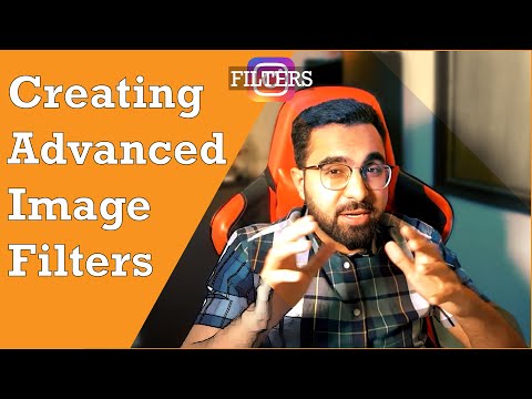
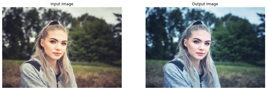
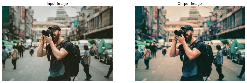
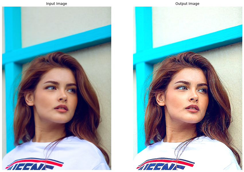
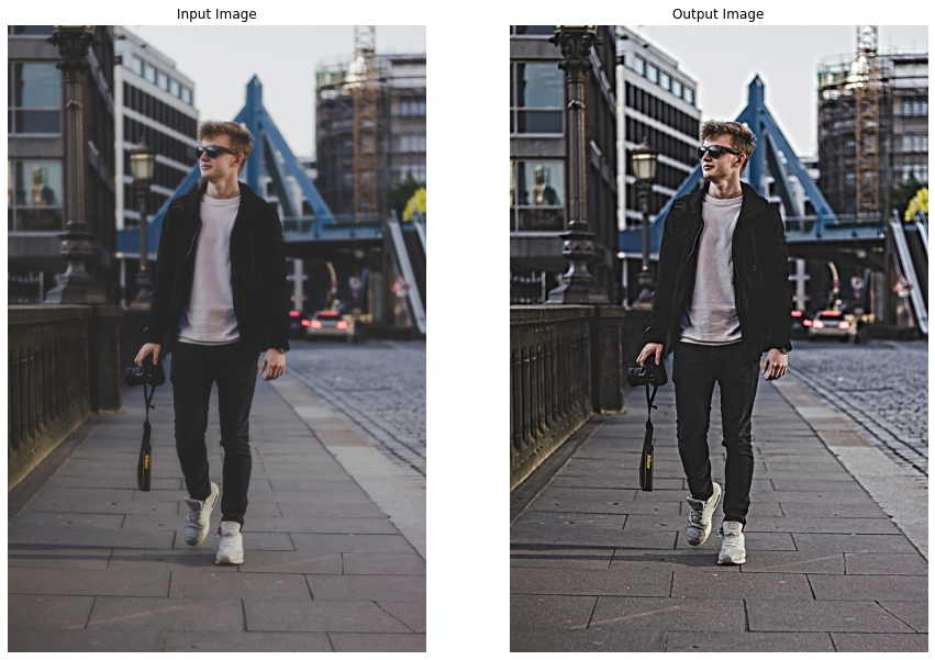
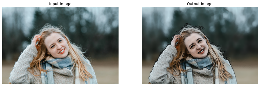
The first filter is gonna be the famous Warm Effect, it absorbs blue cast in images, often caused by electronic flash or outdoor shade, and improves skin tones. This gives a kind of warm look to images that’s why it is called the Warm Effect. To apply this to images and videos, we will create a function applyWarm() that will decrease the pixel intensities of the blue channel and increase the intensities of the red channel of an image/frame by utilizing Look Up tables ( that we learned about in the previous tutorial).
So first, we will have to construct the Look Up Tables required to increase/decrease pixel intensities. For this purpose, we will be using the scipy.interpolate.UnivariateSpline() function to get the required input-output mapping.
# Construct a lookuptable for increasing pixel values.
# We are giving y values for a set of x values.
# And calculating y for [0-255] x values accordingly to the given range.
increase_table = UnivariateSpline(x=[0, 64, 128, 255], y=[0, 75, 155, 255])(range(256))

# Similarly construct a lookuptable for decreasing pixel values.
decrease_table = UnivariateSpline(x=[0, 64, 128, 255], y=[0, 45, 95, 255])(range(256))

# Display the first 10 mappings from the constructed tables.
print(f'First 10 elements from the increase table: \n {increase_table[:10]}\n')
print(f'First 10 elements from the decrease table:: \n {decrease_table[:10]}')
Output:
First 10 elements from the increase table: [7.32204295e-15 1.03827895e+00 2.08227359e+00 3.13191257e+00 4.18712454e+00 5.24783816e+00 6.31398207e+00 7.38548493e+00 8.46227539e+00 9.54428209e+00]
First 10 elements from the decrease table:: [-5.69492230e-15 7.24142824e-01 1.44669675e+00 2.16770636e+00 2.88721627e+00 3.60527107e+00 4.32191535e+00 5.03719372e+00 5.75115076e+00 6.46383109e+00]
Now that we have the Look Up Tables we need, we can move on to transforming the red and blue channel of the image/frame using the function cv2.LUT(). And to split and merge the channels of the image/frame, we will be using the function cv2.split() and cv2.merge() respectively. The applyWarm() function (like every other function in this tutorial) will display the resultant image along with the original image or return the resultant image depending upon the passed arguments.
def applyWarm(image, display=True):
    '''
    This function will create instagram Warm filter like effect on an image.
    Args:
        image:  The image on which the filter is to be applied.
        display: A boolean value that is if set to true the function displays the original image,
                 and the output image, and returns nothing.
    Returns:
        output_image: A copy of the input image with the Warm filter applied.
    '''

    # Split the blue, green, and red channel of the image.
    blue_channel, green_channel, red_channel  = cv2.split(image)

    # Increase red channel intensity using the constructed lookuptable.
    red_channel = cv2.LUT(red_channel, increase_table).astype(np.uint8)

    # Decrease blue channel intensity using the constructed lookuptable.
    blue_channel = cv2.LUT(blue_channel, decrease_table).astype(np.uint8)

    # Merge the blue, green, and red channel.
    output_image = cv2.merge((blue_channel, green_channel, red_channel))

    # Check if the original input image and the output image are specified to be displayed.
    if display:

        # Display the original input image and the output image.
        plt.figure(figsize=[15,15])
        plt.subplot(121);plt.imshow(image[:,:,::-1]);plt.title("Input Image");plt.axis('off');
        plt.subplot(122);plt.imshow(output_image[:,:,::-1]);plt.title("Output Image");plt.axis('off');

    # Otherwise.
    else:

        # Return the output image.
        return output_image
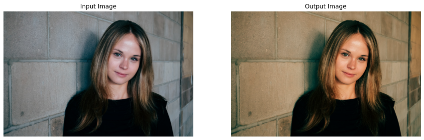
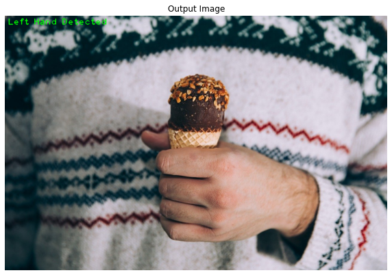
Now, let’s utilize the applyWarm() function created above to apply this warm filter on a few sample images.
# Read a sample image and apply Warm filter on it.
image = cv2.imread('media/sample1.jpg')
applyWarm(image)
# Read another sample image and apply Warm filter on it.
image = cv2.imread('media/sample2.jpg')
applyWarm(image)
Woah! Got the same results as the Instagram warm filter, with just a few lines of code. Now let’s move on to the next one.
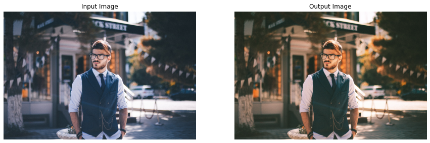
Creating Cold Filter-like Effect
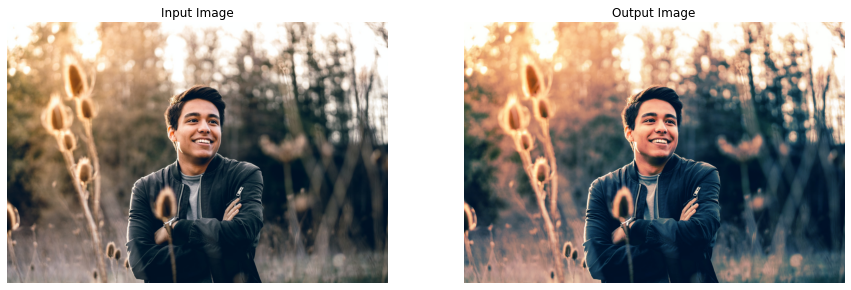
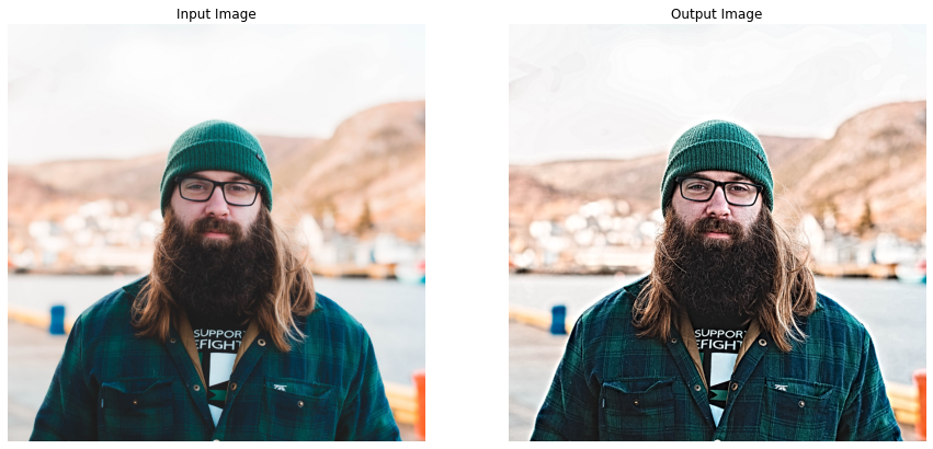
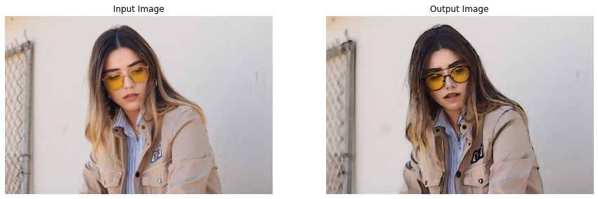
This one is kind of the opposite of the above filter, it gives coldness look to images/videos by increasing the blue cast. To create this filter effect, we will define a function applyCold() that will increase the pixel intensities of the blue channel and decrease the intensities of the red channel of an image/frame by utilizing the same LookUp tables, we had constructed above.
For this one too, we will be using the cv2.split(), cv2.LUT() and cv2.merge() functions to split, transform, and merge the channels.
def applyCold(image, display=True):
    '''
    This function will create instagram Cold filter like effect on an image.
    Args:
        image:  The image on which the filter is to be applied.
        display: A boolean value that is if set to true the function displays the original image,
                 and the output image, and returns nothing.
    Returns:
        output_image: A copy of the input image with the Cold filter applied.
    '''

    # Split the blue, green, and red channel of the image.
    blue_channel, green_channel, red_channel = cv2.split(image)

    # Decrease red channel intensity using the constructed lookuptable.
    red_channel = cv2.LUT(red_channel, decrease_table).astype(np.uint8)

    # Increase blue channel intensity using the constructed lookuptable.
    blue_channel = cv2.LUT(blue_channel, increase_table).astype(np.uint8)

    # Merge the blue, green, and red channel.
    output_image = cv2.merge((blue_channel, green_channel, red_channel))

    # Check if the original input image and the output image are specified to be displayed.
    if display:

        # Display the original input image and the output image.
        plt.figure(figsize=[15,15])
        plt.subplot(121);plt.imshow(image[:,:,::-1]);plt.title("Input Image");plt.axis('off');
        plt.subplot(122);plt.imshow(output_image[:,:,::-1]);plt.title("Output Image");plt.axis('off');

    # Otherwise.
    else:

        # Return the output image.
        return output_image
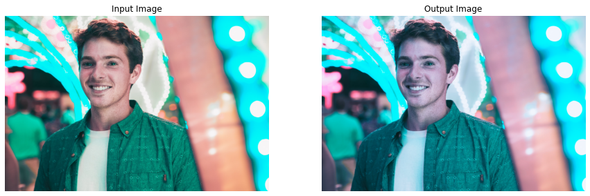
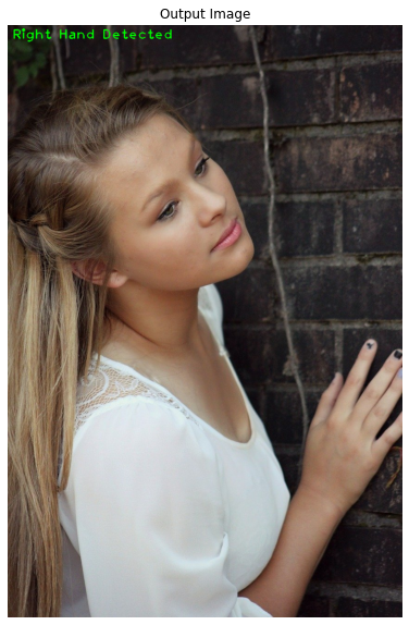
Now we will test this cold filter effect utilizing the applyCold() function on some sample images.
# Read a sample image and apply cold filter on it.
image = cv2.imread('media/sample3.jpg')
applyCold(image)
# Read another sample image and apply cold filter on it.
image = cv2.imread('media/sample4.jpg')
applyCold(image)
Now we’ll use the look up table creat
Nice! Got the expected results for this one too.
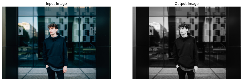
Creating Gotham Filter-like Effect
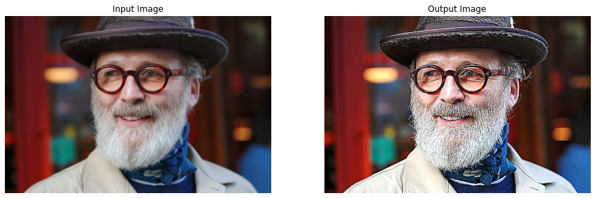
Now the famous Gotham Filter comes in, you must have heard or used this one on Instagram, it gives a warm reddish type look to images. We will try to apply a similar effect to images and videos by creating a function applyGotham(), that will utilize LookUp tables to manipulate image/frame channels in the following manner.
Increase mid-tone contrast of the red channel
Boost the lower-mid values of the blue channel
Decrease the upper-mid values of the blue channel
But again first, we will have to construct the Look Up Tables required to perform the manipulation on the red and blue channels of the image. We will again utilize the scipy.interpolate.UnivariateSpline() function to get the required mapping.
# Construct a lookuptable for increasing midtone contrast.
# Meaning this table will decrease the difference between the midtone values.
# Again we are giving Ys for some Xs and calculating for the remaining ones ([0-255] by using range(256)).
midtone_contrast_increase = UnivariateSpline(x=[0, 25, 51, 76, 102, 128, 153, 178, 204, 229, 255],
                                             y=[0, 13, 25, 51, 76, 128, 178, 204, 229, 242, 255])(range(256))

# Construct a lookuptable for increasing lowermid pixel values.
lowermids_increase = UnivariateSpline(x=[0, 16, 32, 48, 64, 80, 96, 111, 128, 143, 159, 175, 191, 207, 223, 239, 255],
                                      y=[0, 18, 35, 64, 81, 99, 107, 112, 121, 143, 159, 175, 191, 207, 223, 239, 255])(range(256))

# Construct a lookuptable for decreasing uppermid pixel values.
uppermids_decrease = UnivariateSpline(x=[0, 16, 32, 48, 64, 80, 96, 111, 128, 143, 159, 175, 191, 207, 223, 239, 255],
                                      y=[0, 16, 32, 48, 64, 80, 96, 111, 128, 140, 148, 160, 171, 187, 216, 236, 255])(range(256))

# Display the first 10 mappings from the constructed tables.
print(f'First 10 elements from the midtone contrast increase table: \n {midtone_contrast_increase[:10]}\n')
print(f'First 10 elements from the lowermids increase table: \n {lowermids_increase[:10]}\n')
print(f'First 10 elements from the uppermids decrease table:: \n {uppermids_decrease[:10]}')
First 10 elements from the midtone contrast increase table: [0.09416024 0.75724879 1.39938782 2.02149343 2.62448172 3.20926878 3.77677071 4.32790362 4.8635836 5.38472674]
First 10 elements from the lowermids increase table: [0.15030475 1.31080448 2.44957754 3.56865611 4.67007234 5.75585842 6.82804653 7.88866883 8.9397575 9.98334471]
First 10 elements from the uppermids decrease table:: [-0.27440589 0.8349419 1.93606131 3.02916902 4.11448171 5.19221607 6.26258878 7.32581654 8.38211602 9.4317039 ]
Now that we have the required mappings, we can move on to creating the function applyGotham() that will utilize these LookUp tables to apply the required effect.
def applyGotham(image, display=True):
    '''
    This function will create instagram Gotham filter like effect on an image.
    Args:
        image:   The image on which the filter is to be applied.
        display: A boolean value that is if set to true the function displays the original image,
                 and the output image, and returns nothing.
    Returns:
        output_image: A copy of the input image with the Gotham filter applied.
    '''

    # Split the blue, green, and red channel of the image.
    blue_channel, green_channel, red_channel = cv2.split(image)

    # Boost the mid-tone red channel contrast using the constructed lookuptable.
    red_channel = cv2.LUT(red_channel, midtone_contrast_increase).astype(np.uint8)

    # Boost the Blue channel in lower-mids using the constructed lookuptable.
    blue_channel = cv2.LUT(blue_channel, lowermids_increase).astype(np.uint8)

    # Decrease the Blue channel in upper-mids using the constructed lookuptable.
    blue_channel = cv2.LUT(blue_channel, uppermids_decrease).astype(np.uint8)

    # Merge the blue, green, and red channel.
    output_image = cv2.merge((blue_channel, green_channel, red_channel))

    # Check if the original input image and the output image are specified to be displayed.
    if display:

        # Display the original input image and the output image.
        plt.figure(figsize=[15,15])
        plt.subplot(121);plt.imshow(image[:,:,::-1]);plt.title("Input Image");plt.axis('off');
        plt.subplot(122);plt.imshow(output_image[:,:,::-1]);plt.title("Output Image");plt.axis('off');

    # Otherwise.
    else:

        # Return the output image.
        return output_image
Now, let’s test this Gotham effect utilizing the applyGotham() function on a few sample images and visualize the results.
# Read a sample image and apply Gotham filter on it.
image = cv2.imread('media/sample5.jpg')
applyGotham(image)
# Read another sample image and apply Gotham filter on it.
image = cv2.imread('media/sample6.jpg')
applyGotham(image)
Now w
Stunning results! Now, let’s move to a simple one.
Creating Grayscale Filter-like Effect
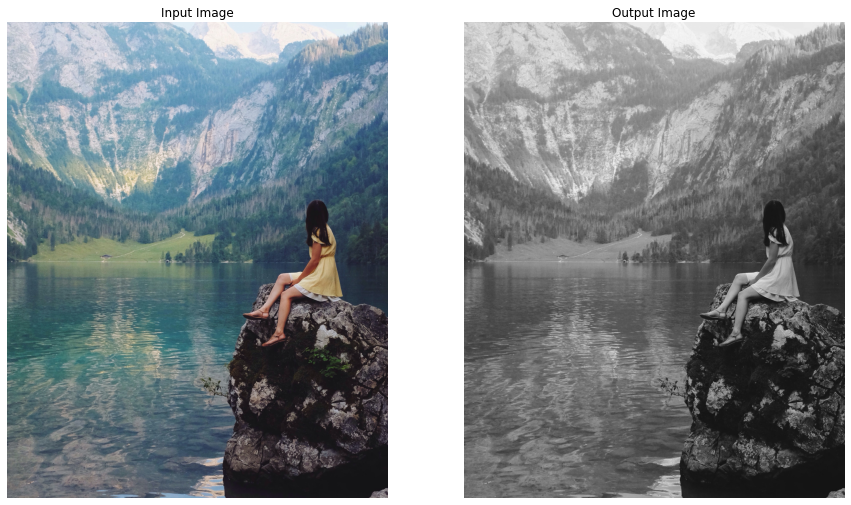
Instagram also has a Grayscale filter also known as 50s TV Effect, it simply converts a (RGB) color image into a Grayscale (black and white) image. We can easily create a similar effect in OpenCV by using the cv2.cvtColor() function. So let’s create a function applyGrayscale() that will utilize cv2.cvtColor() function to apply this Grayscale filter-like effect on images and videos.
def applyGrayscale(image, display=True):
    '''
    This function will create instagram Grayscale filter like effect on an image.
    Args:
        image:  The image on which the filter is to be applied.
        display: A boolean value that is if set to true the function displays the original image,
                 and the output image, and returns nothing.
    Returns:
        output_image: A copy of the input image with the Grayscale filter applied.
    '''

    # Convert the image into the grayscale.
    gray = cv2.cvtColor(image, cv2.COLOR_BGR2GRAY)

    # Merge the grayscale (one-channel) image three times to make it a three-channel image.
    output_image = cv2.merge((gray, gray, gray))

    # Check if the original input image and the output image are specified to be displayed.
    if display:

        # Display the original input image and the output image.
        plt.figure(figsize=[15,15])
        plt.subplot(121);plt.imshow(image[:,:,::-1]);plt.title("Input Image");plt.axis('off');
        plt.subplot(122);plt.imshow(output_image[:,:,::-1]);plt.title("Output Image");plt.axis('off');

    # Otherwise.
    else:

        # Return the output image.
        return output_image
Now let’s utilize this applyGrayscale() function to apply the grayscale effect on a few sample images and display the results.
# Read a sample image| and apply Grayscale filter on it.
image = cv2.imread('media/sample7.jpg')
applyGrayscale(image)
# Read another sample image and apply Grayscale filter on it.
image = cv2.imread('media/sample8.jpg')
applyGrayscale(image)
Cool! Working as expected. Let’s move on to the next one.
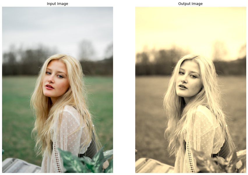
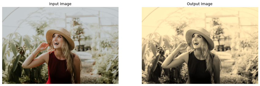
Creating Sepia Filter-like Effect
I think this one is the most famous among all the filters we are creating today. This gives a warm reddish-brown vintage effect to images which makes the images look a bit ancient which is really cool. To apply this effect, we will create a function applySepia() that will utilize the cv2.transform() function and the fixed sepia matrix (standardized to create this effect, that you can easily find online) to serve the purpose.
def applySepia(image, display=True):
    '''
    This function will create instagram Sepia filter like effect on an image.
    Args:
        image:  The image on which the filter is to be applied.
        display: A boolean value that is if set to true the function displays the original image,
                 and the output image, and returns nothing.
    Returns:
        output_image: A copy of the input image with the Sepia filter applied.
    '''

    # Convert the image into float type to prevent loss during operations.
    image_float = np.array(image, dtype=np.float64)


    # Manually transform the image to get the idea of exactly whats happening.
    ##################################################################################################

    # Split the blue, green, and red channel of the image.
    blue_channel, green_channel, red_channel = cv2.split(image_float)

    # Apply the Sepia filter by perform the matrix multiplication between
    # the image and the sepia matrix.
    output_blue = (red_channel * .272) + (green_channel *.534) + (blue_channel * .131)
    output_green = (red_channel * .349) + (green_channel *.686) + (blue_channel * .168)
    output_red = (red_channel * .393) + (green_channel *.769) + (blue_channel * .189)

    # Merge the blue, green, and red channel.
    output_image = cv2.merge((output_blue, output_green, output_red))

    ##################################################################################################


        # OR Either create this effect by using OpenCV matrix transformation function.
    ##################################################################################################

    # Get the sepia matrix for BGR colorspace images.
    sepia_matrix = np.matrix([[.272, .534, .131],
                              [.349, .686, .168],
                              [.393, .769, .189]])

    # Apply the Sepia filter by perform the matrix multiplication between
    # the image and the sepia matrix.
    #output_image = cv2.transform(src=image_float, m=sepia_matrix)

    ##################################################################################################


    # Set the values > 255 to 255.
    output_image[output_image > 255] = 255

    # Convert the image back to uint8 type.
    output_image =  np.array(output_image, dtype=np.uint8)

    # Check if the original input image and the output image are specified to be displayed.
    if display:

        # Display the original input image and the output image.
        plt.figure(figsize=[15,15])
        plt.subplot(121);plt.imshow(image[:,:,::-1]);plt.title("Input Image");plt.axis('off');
        plt.subplot(122);plt.imshow(output_image[:,:,::-1]);plt.title("Output Image");plt.axis('off');

    # Otherwise.
    else:

        # Return the output image.
        return output_image
Now let’s check this sepia effect by utilizing the applySepia() function on a few sample images.
# Read a sample image and apply Sepia filter on it.
image = cv2.imread('media/sample9.jpg')
applySepia(image)
# Read another sample image and apply Sepia filter on it.
image = cv2.imread('media/sample18.jpg')
applySepia(image)
Spectacular results! Reminds me of the movies, I used to watch in my childhood ( Yes, I am that old 😜 ).
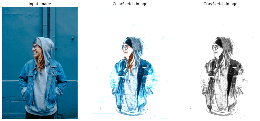
Creating Pencil Sketch Filter-like Effect
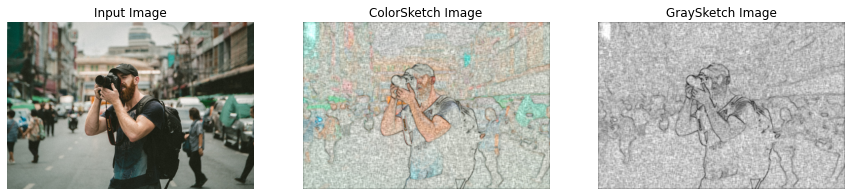
The next one is the Pencil Sketch Filter, creating a Pencil Sketch manually requires hours of hard work but luckily in OpenCV, we can do this in just one line of code by using the function cv2.pencilSketch() that give a pencil sketch-like effect to images. So lets create a function applyPencilSketch() to convert images/videos into Pencil Sketches utilizing the cv2.pencilSketch() function.
We will use the following funciton to applythe pencil sketch filter, this function retruns a grayscale sketch and a colored sketch of the image
This filter is a type of edge preserving filter, these filters have 2 Objectives, one is to give more weightage to pixels closer so that the blurring can be meaningfull and second to average only the similar intensity valued pixels to avoid the edges, so in this both of these objectives are controled by the two following parameters.
sigma_s Just like sigma in other smoothing filters this sigma value controls the area of the neighbourhood (Has Range between 0-200)
sigma_r This param controls the how dissimilar colors within the neighborhood will be averaged. For example a larger value will restrcit color variation and it will enforce that constant color stays throughout. (Has Range between 0-1)
shade_factor This has range 0-0.1 and controls how bright the final output will be by scaling the intensity.
def applyPencilSketch(image, display=True):
    '''
    This function will create instagram Pencil Sketch filter like effect on an image.
    Args:
        image:  The image on which the filter is to be applied.
        display: A boolean value that is if set to true the function displays the original image,
                 and the output image, and returns nothing.
    Returns:
        output_image: A copy of the input image with the Pencil Sketch filter applied.
    '''

    # Apply Pencil Sketch effect on the image.
    gray_sketch, color_sketch = cv2.pencilSketch(image, sigma_s=20, sigma_r=0.5, shade_factor=0.02)

    # Check if the original input image and the output image are specified to be displayed.
    if display:

        # Display the original input image and the output image.
        plt.figure(figsize=[15,15])
        plt.subplot(131);plt.imshow(image[:,:,::-1]);plt.title("Input Image");plt.axis('off');
        plt.subplot(132);plt.imshow(color_sketch[:,:,::-1]);plt.title("ColorSketch Image");plt.axis('off');
        plt.subplot(133);plt.imshow(gray_sketch, cmap='gray');plt.title("GraySketch Image");plt.axis('off');

    # Otherwise.
    else:

        # Return the output image.
        return color_sketch
Now we will apply this pencil sketch effect by utilizing the applyPencilSketch() function on a few sample images and visualize the results.
# Read a sample image and apply PencilSketch filter on it.
image = cv2.imread('media/sample11.jpg')
applyPencilSketch(image)
Now let’s check how the changeIntensity() functi
# Read another sample image and apply PencilSketch filter on it.
image = cv2.imread('media/sample5.jpg')
applyPencilSketch(image)
Amazing right? we created this effect with just a single line of code. So now, instead of spending hours manually sketching someone or something, you can take an image and apply this effect on it to get the results in seconds. And you can further tune the parameters of the cv2.pencilSketch() function to get even better results.
Creating Sharpening Filter-like Effect
Now let’s try to create the Sharpening Effect, this enhances the clearness of an image/video and decreases the blurriness which gives a new interesting look to the image/video. For this we will create a function applySharpening() that will utilize the cv2.filter2D() function to give the required effect to an image/frame passed to it.
 def applySharpening(image, display=True):
    '''
    This function will create the Sharpening filter like effect on an image.
    Args:
        image:  The image on which the filter is to be applied.
        display: A boolean value that is if set to true the function displays the original image,
                 and the output image, and returns nothing.
    Returns:
        output_image: A copy of the input image with the Sharpening filter applied.
    '''

    # Get the kernel required for the sharpening effect.
    sharpening_kernel = np.array([[-1, -1, -1],
                                  [-1, 9.2, -1],
                                  [-1, -1, -1]])

    # Apply the sharpening filter on the image.
    output_image = cv2.filter2D(src=image, ddepth=-1,
                                kernel=sharpening_kernel)

    # Check if the original input image and the output image are specified to be displayed.
    if display:

        # Display the original input image and the output image.
        plt.figure(figsize=[15,15])
        plt.subplot(121);plt.imshow(image[:,:,::-1]);plt.title("Input Image");plt.axis('off');
        plt.subplot(122);plt.imshow(output_image[:,:,::-1]);plt.title("Output Image");plt.axis('off');

    # Otherwise.
    else:

        # Return the output image.
        return output_image
Now, let’s see this in action utilizing the applySharpening() function created above on a few sample images.
# Read a sample image and apply Sharpening filter on it.
image = cv2.imread('media/sample12.jpg')
applySharpening(image)
# Read another sample image and apply Sharpening filter on it.
image = cv2.imread('media/sample13.jpg')
applySharpening(image)
Nice! this filter makes the original images look as if they are out of focus (blur).
Creating a Detail Enhancing Filter
Now this Filter is another type of edge preserving fitler and has the same parameters as the pencil sketch filter.This filter intensifies the details in images/videos, we’ll be using the function called cv2.detailEnhance(). let’s start by creating the a wrapper function applyDetailEnhancing(), that will utilize the cv2.detailEnhance() function to apply the needed effect.
def applyDetailEnhancing(image, display=True):
    '''
    This function will create the HDR filter like effect on an image.
    Args:
        image:  The image on which the filter is to be applied.
        display: A boolean value that is if set to true the function displays the original image,
                 and the output image, and returns nothing.
    Returns:
        output_image: A copy of the input image with the HDR filter applied.
    '''

    # Apply the detail enhancing effect by enhancing the details of the image.
    output_image = cv2.detailEnhance(image, sigma_s=15, sigma_r=0.15)

    # Check if the original input image and the output image are specified to be displayed.
    if display:

        # Display the original input image and the output image.
        plt.figure(figsize=[15,15])
        plt.subplot(121);plt.imshow(image[:,:,::-1]);plt.title("Input Image");plt.axis('off');
        plt.subplot(122);plt.imshow(output_image[:,:,::-1]);plt.title("Output Image");plt.axis('off');

    # Otherwise.
    else:

        # Return the output image.
        return output_image
Now, let’s test the function applyDetailEnhancing() created above on a few sample images.
# Read a sample image and apply Detail Enhancing filter on it.
image = cv2.imread('media/sample14.jpg')
applyDetailEnhancing(image)
# Read another sample image and apply Detail Enhancing filter on it.
image = cv2.imread('media/sample15.jpg')
applyDetailEnhancing(image)
Satisfying results! let’s move on to the next one.
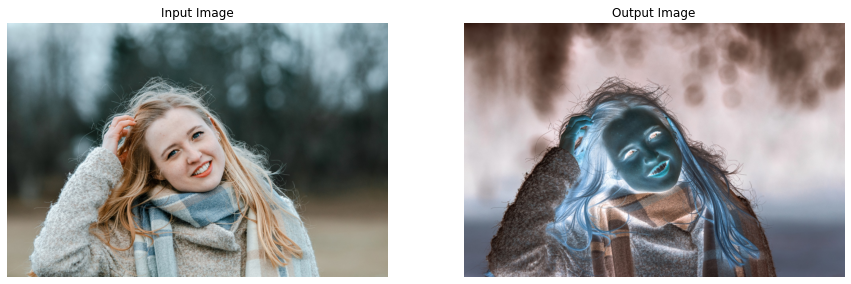
Creating Invert Filter-like Effect
This filter inverts the colors in images/videos meaning changes darkish colors into light and vice versa, which gives a very interesting look to images/videos. This can be accomplished using multiple approaches we can either utilize a LookUp table to perform the required transformation or subtract the image by 255 and take absolute of the results or just simply use the OpenCV function cv2.bitwise_not(). Let’s create a function applyInvert() to serve the purpose.
def applyInvert(image, display=True):
    '''
    This function will create the Invert filter like effect on an image.
    Args:
        image:  The image on which the filter is to be applied.
        display: A boolean value that is if set to true the function displays the original image,
                 and the output image, and returns nothing.
    Returns:
        output_image: A copy of the input image with the Invert filter applied.
    '''

    # Apply the Invert Filter on the image.
    output_image = cv2.bitwise_not(image)

    # Check if the original input image and the output image are specified to be displayed.
    if display:

        # Display the original input image and the output image.
        plt.figure(figsize=[15,15])
        plt.subplot(121);plt.imshow(image[:,:,::-1]);plt.title("Input Image");plt.axis('off');
        plt.subplot(122);plt.imshow(output_image[:,:,::-1]);plt.title("Output Image");plt.axis('off');

    # Otherwise.
    else:

        # Return the output image.
        return output_image
Let’s check this effect on a few sample images utilizing the applyInvert() function.
# Read a sample image and apply invert filter on it.
image = cv2.imread('media/sample16.jpg')
applyInvert(image)
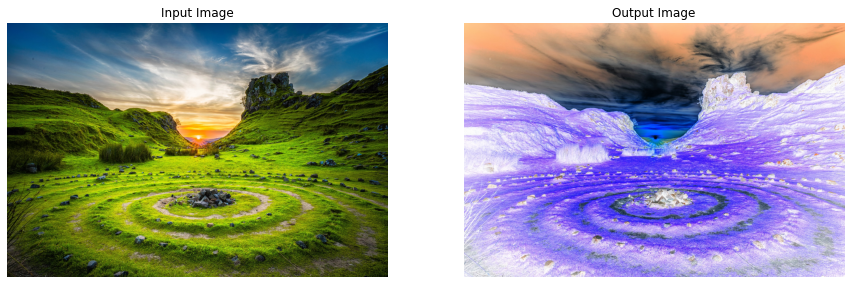
Looks a little scary, lets’s try it on a few landscape images.
# Read a landscape image and apply invert filter on it.
image = cv2.imread('media/sample19.jpg')
applyInvert(image)
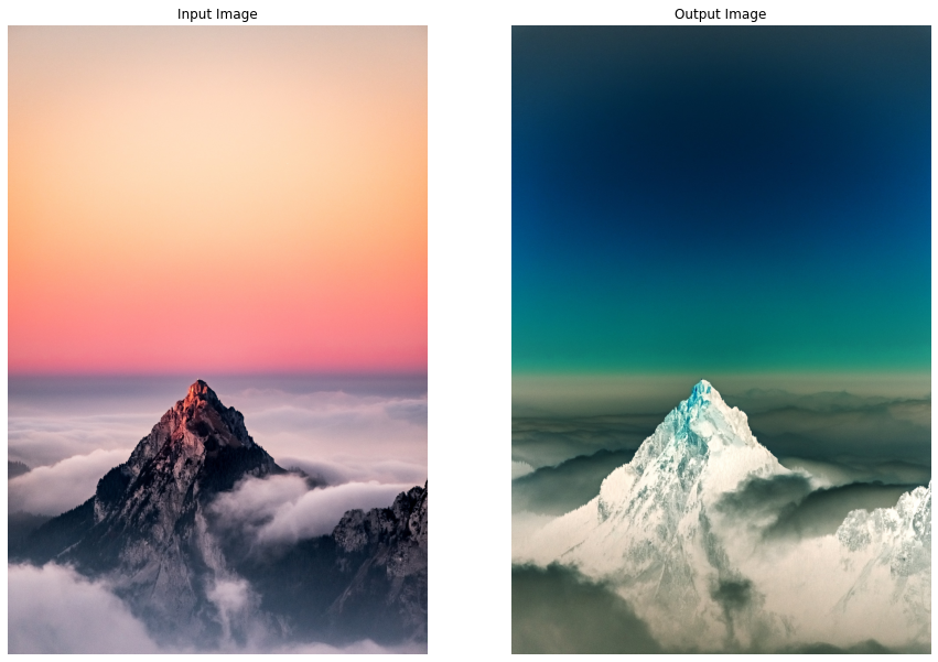
# Read another landscape image and apply invert filter on it.
image = cv2.imread('media/sample20.jpg')
applyInvert(image)
Interesting effect! but I will definitely not recommend using this one on your own images, except if your intention is to scare someone xD.
Creating Stylization Filter-like Effect
Now let’s move on to the final one, which gives a painting-like effect to images. We will create a function applyStylization() that will utilize the cv2.stylization() function to apply this effect on images and videos. This one too will only need a single line of code.
def applyStylization(image, display=True):
    '''
    This function will create instagram cartoon-paint filter like effect on an image.
    Args:
        image:  The image on which the filter is to be applied.
        display: A boolean value that is if set to true the function displays the original image,
                 and the output image, and returns nothing.
    Returns:
        output_image: A copy of the input image with the cartoon-paint filter applied.
    '''

    # Apply stylization effect on the image.
    output_image = cv2.stylization(image, sigma_s=15, sigma_r=0.55)

    # Check if the original input image and the output image are specified to be displayed.
    if display:

        # Display the original input image and the output image.
        plt.figure(figsize=[15,15])
        plt.subplot(121);plt.imshow(image[:,:,::-1]);plt.title("Input Image");plt.axis('off');
        plt.subplot(122);plt.imshow(output_image[:,:,::-1]);plt.title("Output Image");plt.axis('off');

    # Otherwise.
    else:

        # Return the output image.
        return output_image
Now, as done for every other filter, we will utilize the function applyStylization() to test this effect on a few sample images.
# Read a sample image and apply Stylization filter on it.
image = cv2.imread('media/sample16.jpg')
applyStylization(image)
# Read another sample image and apply Stylization filter on it.
image = cv2.imread('media/sample17.jpg')
applyStylization(image)
Again got fascinating results! Wasn’t that fun to see how simple it is to create all these effects?
Apply Instagram Filters On a Real-Time Web-cam Feed
Now that we have created the filters and have tested them on images, let’s move to apply these on a real-time webcam feed, first, we will have to create a mouse event callback function mouseCallback(), similar to the one we had created for the Color Filters in the previous tutorial, the function will allow us to select the filter to apply, and capture and store images into the disk by utilizing mouse events in real-time.
def mouseCallback(event, x, y, flags, userdata):
    '''
    This function will update the filter to apply on the frame and capture images based on different mouse events.
    Args:
        event:    The mouse event that is captured.
        x:        The x-coordinate of the mouse pointer position on the window.
        y:        The y-coordinate of the mouse pointer position on the window.
        flags:    It is one of the MouseEventFlags constants.
        userdata: The parameter passed from the `cv2.setMouseCallback()` function.
    '''
    #  Access the filter applied, and capture image state variable.
    global filter_applied, capture_image

    # Check if the left mouse button is pressed.
    if event == cv2.EVENT_LBUTTONDOWN:

        # Check if the mouse pointer is over the camera icon ROI.
        if y >= (frame_height-10)-camera_icon_height and \
        x >= (frame_width//2-camera_icon_width//2) and \
        x <= (frame_width//2+camera_icon_width//2):

            # Update the image capture state to True.
            capture_image = True

        # Check if the mouse pointer y-coordinate is over the filters ROI.
        elif y <= 10+preview_height:

            # Check if the mouse pointer x-coordinate is over the Warm filter ROI.
            if x>(int(frame_width//11.6)-preview_width//2) and \
            x<(int(frame_width//11.6)-preview_width//2)+preview_width:

                # Update the filter applied variable value to Warm.
                filter_applied = 'Warm'

            # Check if the mouse pointer x-coordinate is over the Cold filter ROI.
            elif x>(int(frame_width//5.9)-preview_width//2) and \
            x<(int(frame_width//5.9)-preview_width//2)+preview_width:

                # Update the filter applied variable value to Cold.
                filter_applied = 'Cold'

            # Check if the mouse pointer x-coordinate is over the Gotham filter ROI.
            elif x>(int(frame_width//3.97)-preview_width//2) and \
            x<(int(frame_width//3.97)-preview_width//2)+preview_width:

                # Update the filter applied variable value to Gotham.
                filter_applied = 'Gotham'

            # Check if the mouse pointer x-coordinate is over the Grayscale filter ROI.
            elif x>(int(frame_width//2.99)-preview_width//2) and \
            x<(int(frame_width//2.99)-preview_width//2)+preview_width:

                # Update the filter applied variable value to Grayscale.
                filter_applied = 'Grayscale'

            # Check if the mouse pointer x-coordinate is over the Sepia filter ROI.
            elif x>(int(frame_width//2.395)-preview_width//2) and \
            x<(int(frame_width//2.395)-preview_width//2)+preview_width:

                # Update the filter applied variable value to Sepia.
                filter_applied = 'Sepia'

            # Check if the mouse pointer x-coordinate is over the Normal filter ROI.
            elif x>(int(frame_width//2)-preview_width//2) and \
            x<(int(frame_width//2)-preview_width//2)+preview_width:

                # Update the filter applied variable value to Normal.
                filter_applied = 'Normal'

            # Check if the mouse pointer x-coordinate is over the Pencil Sketch filter ROI.
            elif x>(frame_width//1.715-preview_width//2) and \
            x<(frame_width//1.715-preview_width//2)+preview_width:

                # Update the filter applied variable value to Pencil Sketch.
                filter_applied = 'Pencil Sketch'

            # Check if the mouse pointer x-coordinate is over the Sharpening filter ROI.
            elif x>(int(frame_width//1.501)-preview_width//2) and \
            x<(int(frame_width//1.501)-preview_width//2)+preview_width:

                # Update the filter applied variable value to Sharpening.
                filter_applied = 'Sharpening'

            # Check if the mouse pointer x-coordinate is over the Invert filter ROI.
            elif x>(int(frame_width//1.335)-preview_width//2) and \
            x<(int(frame_width//1.335)-preview_width//2)+preview_width:

                # Update the filter applied variable value to Invert.
                filter_applied = 'Invert'

            # Check if the mouse pointer x-coordinate is over the Detail Enhancing filter ROI.
            elif x>(int(frame_width//1.202)-preview_width//2) and \
            x<(int(frame_width//1.202)-preview_width//2)+preview_width:

                # Update the filter applied variable value to Detail Enhancing.
                filter_applied = 'Detail Enhancing'

            # Check if the mouse pointer x-coordinate is over the Stylization filter ROI.
            elif x>(int(frame_width//1.094)-preview_width//2) and \
            x<(int(frame_width//1.094)-preview_width//2)+preview_width:

                # Update the filter applied variable value to Stylization.
                filter_applied = 'Stylization'
Now that we have a mouse event callback function mouseCallback() to select a filter to apply, we will create another function applySelectedFilter() that we will need, to check which filter is selected at the moment and apply that filter to the image/frame in real-time.
def applySelectedFilter(image, filter_applied):
    '''
    This function will apply the selected filter on an image.
    Args:
        image:          The image on which the selected filter is to be applied.
        filter_applied: The name of the filter selected by the user.
    Returns:
        output_image: A copy of the input image with the selected filter applied.
    '''

    # Check if the specified filter to apply, is the Warm filter.
    if filter_applied == 'Warm':

        # Apply the Warm Filter on the image.
        output_image = applyWarm(image, display=False)

    # Check if the specified filter to apply, is the Cold filter.
    elif filter_applied == 'Cold':

        # Apply the Cold Filter on the image.
        output_image = applyCold(image, display=False)

    # Check if the specified filter to apply, is the Gotham filter.
    elif filter_applied == 'Gotham':

        # Apply the Gotham Filter on the image.
        output_image = applyGotham(image, display=False)

     # Check if the specified filter to apply, is the Grayscale filter.
    elif filter_applied == 'Grayscale':

        # Apply the Grayscale Filter on the image.
        output_image = applyGrayscale(image, display=False)

    # Check if the specified filter to apply, is the Sepia filter.
    if filter_applied == 'Sepia':

        # Apply the Sepia Filter on the image.
        output_image = applySepia(image, display=False)

    # Check if the specified filter to apply, is the Pencil Sketch filter.
    elif filter_applied == 'Pencil Sketch':

        # Apply the Pencil Sketch Filter on the image.
        output_image = applyPencilSketch(image, display=False)

    # Check if the specified filter to apply, is the Sharpening filter.
    elif filter_applied == 'Sharpening':

        # Apply the Sharpening Filter on the image.
        output_image = applySharpening(image, display=False)

    # Check if the specified filter to apply, is the Invert filter.
    elif filter_applied == 'Invert':

        # Apply the Invert Filter on the image.
        output_image = applyInvert(image, display=False)

    # Check if the specified filter to apply, is the Detail Enhancing filter.
    elif filter_applied == 'Detail Enhancing':

        # Apply the Detail Enhancing Filter on the image.
        output_image = applyDetailEnhancing(image, display=False)

    # Check if the specified filter to apply, is the Stylization filter.
    elif filter_applied == 'Stylization':

        # Apply the Stylization Filter on the image.
        output_image = applyStylization(image, display=False)

    # Return the image with the selected filter applied.`
    return output_image
Now that we will the required functions, let’s test the filters on a real-time webcam feed, we will be switching between the filters by utilizing the mouseCallback() and applySelectedFilter() functions created above and will overlay a Camera ROI over the frame and allow the user to capture images with the selected filter applied, by clicking on the Camera ROI in real-time.
# Initialize the VideoCapture object to read from the webcam.
camera_video = cv2.VideoCapture(1, cv2.CAP_DSHOW)
camera_video.set(3,1280)
camera_video.set(4,960)

# Create a named resizable window.
cv2.namedWindow('Instagram Filters', cv2.WINDOW_NORMAL)

# Attach the mouse callback function to the window.
cv2.setMouseCallback('Instagram Filters', mouseCallback)

# Initialize a variable to store the current applied filter.
filter_applied = 'Normal'

# Initialize a variable to store the copies of the frame
# with the filters applied.
filters = None

# Initialize the pygame modules and load the image-capture music file.
pygame.init()
pygame.mixer.music.load("media/camerasound.mp3")

# Initialize a variable to store the image capture state.
capture_image = False

# Initialize a variable to store a camera icon image.
camera_icon = None

# Iterate until the webcam is accessed successfully.
while camera_video.isOpened():

    # Read a frame.
    ok, frame = camera_video.read()

    # Check if frame is not read properly then
    # continue to the next iteration to read the next frame.
    if not ok:
        continue

    # Get the height and width of the frame of the webcam video.
    frame_height, frame_width, _ = frame.shape

    # Flip the frame horizontally for natural (selfie-view) visualization.
    frame = cv2.flip(frame, 1)

    # Check if the filters variable doesnot contain the filters.
    if not(filters):

        # Update the filters variable to store a dictionary containing multiple
        # copies of the frame with all the filters applied.
        filters = {'Normal': frame.copy(), 'Warm' : applyWarm(frame, display=False),
                   'Cold'  :applyCold(frame, display=False),
                   'Gotham' : applyGotham(frame, display=False),
                   'Grayscale' : applyGrayscale(frame, display=False),
                   'Sepia' : applySepia(frame, display=False),
                   'Pencil Sketch' : applyPencilSketch(frame, display=False),
                   'Sharpening': applySharpening(frame, display=False),
                   'Invert': applyInvert(frame, display=False),
                   'Detail Enhancing': applyDetailEnhancing(frame, display=False),
                   'Stylization': applyStylization(frame, display=False)}

    # Initialize a list to store the previews of the filters.
    filters_previews = []

    # Iterate over the filters dictionary.
    for filter_name, filtered_frame in filters.items():

        # Check if the filter we are iterating upon, is applied.
        if filter_applied == filter_name:

            # Set color to green.
            # This will be the border color of the filter preview.
            # And will be green for the filter applied and white for the other filters.
            color = (0,255,0)

        # Otherwise.
        else:

            # Set color to white.
            color = (255,255,255)

        # Make a border around the filter we are iterating upon.
        filter_preview = cv2.copyMakeBorder(src=filtered_frame, top=100, bottom=100,
                                            left=10, right=10, borderType=cv2.BORDER_CONSTANT,
                                            value=color)

        # Resize the preview to the 1/12th of its current width and height.
        filter_preview = cv2.resize(filter_preview, (frame_width//12,frame_height//12))

        # Append the filter preview into the list.
        filters_previews.append(filter_preview)

    # Get the new height and width of the previews.
    preview_height, preview_width, _ = filters_previews[0].shape

    # Check if any filter is selected.
    if filter_applied != 'Normal':

        # Apply the selected Filter on the frame.
        frame = applySelectedFilter(frame, filter_applied)

     # Check if the image capture state is True.
    if capture_image:

        # Capture an image and store it in the disk.
        cv2.imwrite('Captured_Image.png', frame)

        # Display a black image.
        cv2.imshow('Instagram Filters', np.zeros((frame_height, frame_width)))

        # Play the image capture music to indicate that an image is captured and wait for 100 milliseconds.
        pygame.mixer.music.play()
        cv2.waitKey(100)

        # Display the captured image.
        plt.close();plt.figure(figsize=[10, 10])
        plt.imshow(frame[:,:,::-1]);plt.title("Captured Image");plt.axis('off');

        # Update the image capture state to False.
        capture_image = False

    # Check if the camera icon variable doesnot contain the camera icon image.
    if not(camera_icon):

        # Read a camera icon png image with its blue, green, red, and alpha channel.
        camera_iconBGRA = cv2.imread('media/cameraicon.png', cv2.IMREAD_UNCHANGED)

        # Resize the camera icon image to the 1/12th of the frame width,
        # while keeping the aspect ratio constant.
        camera_iconBGRA = cv2.resize(camera_iconBGRA,
                                     (frame_width//12,
                                      int(((frame_width//12)/camera_iconBGRA.shape[1])*camera_iconBGRA.shape[0])))

        # Get the new height and width of the camera icon image.
        camera_icon_height, camera_icon_width, _ = camera_iconBGRA.shape

        # Get the first three-channels (BGR) of the camera icon image.
        camera_iconBGR  = camera_iconBGRA[:,:,:-1]

        # Get the alpha channel of the camera icon.
        camera_icon_alpha =  camera_iconBGRA[:,:,-1]

    # Get the region of interest of the frame where the camera icon image will be placed.
    frame_roi = frame[(frame_height-10)-camera_icon_height: (frame_height-10),
                      (frame_width//2-camera_icon_width//2): \
                      (frame_width//2-camera_icon_width//2)+camera_icon_width]

    # Overlay the camera icon over the frame by updating the pixel values of the frame
    # at the indexes where the alpha channel of the camera icon image has the value 255.
    frame_roi[camera_icon_alpha==255] = camera_iconBGR[camera_icon_alpha==255]

    # Overlay the resized preview filter images over the frame by updating
    # its pixel values in the region of interest.
    #######################################################################################

    # Overlay the Warm Filter preview on the frame.
    frame[10: 10+preview_height,
          (int(frame_width//11.6)-preview_width//2): \
          (int(frame_width//11.6)-preview_width//2)+preview_width] = filters_previews[1]

    # Overlay the Cold Filter preview on the frame.
    frame[10: 10+preview_height,
          (int(frame_width//5.9)-preview_width//2): \
          (int(frame_width//5.9)-preview_width//2)+preview_width] = filters_previews[2]

    # Overlay the Gotham Filter preview on the frame.
    frame[10: 10+preview_height,
          (int(frame_width//3.97)-preview_width//2): \
          (int(frame_width//3.97)-preview_width//2)+preview_width] = filters_previews[3]


    # Overlay the Grayscale Filter preview on the frame.
    frame[10: 10+preview_height,
          (int(frame_width//2.99)-preview_width//2): \
          (int(frame_width//2.99)-preview_width//2)+preview_width] = filters_previews[4]

    # Overlay the Sepia Filter preview on the frame.
    frame[10: 10+preview_height,
          (int(frame_width//2.395)-preview_width//2): \
          (int(frame_width//2.395)-preview_width//2)+preview_width] = filters_previews[5]

    # Overlay the Normal frame (no filter) preview on the frame.
    frame[10: 10+preview_height,
          (frame_width//2-preview_width//2): \
          (frame_width//2-preview_width//2)+preview_width] = filters_previews[0]

    # Overlay the Pencil Sketch Filter preview on the frame.
    frame[10: 10+preview_height,
          (int(frame_width//1.715)-preview_width//2): \
          (int(frame_width//1.715)-preview_width//2)+preview_width]=filters_previews[6]

    # Overlay the Sharpening Filter preview on the frame.
    frame[10: 10+preview_height,
          (int(frame_width//1.501)-preview_width//2): \
          (int(frame_width//1.501)-preview_width//2)+preview_width]=filters_previews[7]

    # Overlay the Invert Filter preview on the frame.
    frame[10: 10+preview_height,
          (int(frame_width//1.335)-preview_width//2): \
          (int(frame_width//1.335)-preview_width//2)+preview_width]=filters_previews[8]

    # Overlay the Detail Enhancing Filter preview on the frame.
    frame[10: 10+preview_height,
          (int(frame_width//1.202)-preview_width//2): \
          (int(frame_width//1.202)-preview_width//2)+preview_width]=filters_previews[9]

    # Overlay the Stylization Filter preview on the frame.
    frame[10: 10+preview_height,
          (int(frame_width//1.094)-preview_width//2): \
          (int(frame_width//1.094)-preview_width//2)+preview_width]=filters_previews[10]

    #######################################################################################

    # Display the frame.
    cv2.imshow('Instagram Filters', frame)

    # Wait for 1ms. If a key is pressed, retreive the ASCII code of the key.
    k = cv2.waitKey(1) & 0xFF

    # Check if 'ESC' is pressed and break the loop.
    if(k == 27):
        break

# Release the VideoCapture Object and close the windows.
camera_video.release()
cv2.destroyAllWindows()
Output Video:
Awesome! working as expected on the videos too.
Assignment (Optional)
Create your own Filter with an appropriate name by playing around with the techniques you have learned in this tutorial, and share the results with me in the comments section.
In today’s tutorial, we have covered several advanced image processing techniques and then utilized these concepts to create 10 different fascinating Instagram filters-like effects on images and videos.
This concludes the Creating Instagram Filters series, throughout the series we learned a ton of interesting concepts. In the first post, we learned all about using Mouse and TrackBars events in OpenCV, in the second post we learned to work with Lookup Tables in OpenCV and how to create color filters with it, and in this tutorial, we went even further and created more interesting color filters and other types of effects.
If you have found the series useful, do let me know in the comments section, I might publish some other very cool posts on image filters using deep learning. We also provide AI Consulting at Bleed AI Solutions, by building highly optimized and scalable bleeding-edge solutions for our clients so feel free to contact us if you have a problem or project that demands a cutting-edge AI/CV solution.
In the previous episode of the Computer Vision For Everyone (CVFE) course, we discussed different branches of machine learning in detail with examples. Now in today’s episode, we’ll further dive in, by learning about some interesting hybrid branches of AI.
We’ll also learn about AI industries, AI applications, applied AI fields, and a lot more, including how everything is connected with each other. Believe me, this is one tutorial that will tie a lot of AI Concepts together that you’ve heard out there, you don’t want to skip it.
By the way, this is the final part of Artificial Intelligence 4 levels of explanation. All the four posts are titled as:
Hybrid Branches of AI with Complete Overview of the Field | Artificial Intelligence Part 4/4 (Episode 6 | CVFE) (Current tutorial)
This tutorial is built on top of the previous ones so make sure to go over those parts first if you haven’t already, especially the last one in which I had covered the core branches of machine learning. If you already know about a high-level overview of supervised, unsupervised, and reinforcement learning then you’re all good.
Alright, so without further ado, let’s get into it.
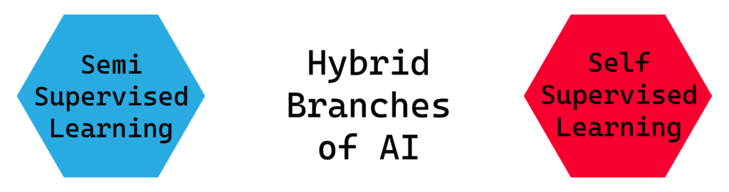
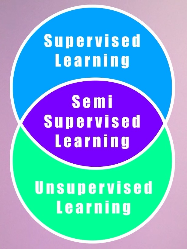
We have already learned about Core ML branches, Supervised Learning, Unsupervised Learning, and Reinforcement Learning, so now it’s time to explore hybrid branches, which use a mix of techniques from these three core branches. The two most useful hybrid fields are; Semi-Supervised Learning and Self-Supervised Learning. And both of these hybrid fields actually fall in a category of Machine Learning called Weak Supervision. Don’t worry I’ll explain all the terms.
The aim of hybrid fields like Semi-Supervised and Self-Supervised learning is to come up with approaches that bypass the time-consuming manual data labeling process involved in Supervised Learning.
So here’s the thing supervised learning is the most popular category of machine learning and it has the most applications in the industry and In today’s era where an everyday people are uploading images, text, blogposts in huge quantities, we’re at a point where we could train supervised models for almost anything with reasonable accuracy but here’s the issue, even though we have lots and lots of data, it’s actually very costly and time-consuming to label all of it.
So what we need to do is somehow use methods that are as effective as supervised learning but don’t require us, humans, to label all the data. This is where these hybrid fields come up, and almost all of these are essentially trying to solve the same problem.
There are some other approaches out there as well, like the Multi-Instance Learning and some others that also, but we won’t be going over those in this tutorial as Semi-Supervised and Self-Supervised Learning are more frequently used than the other approaches.
Semi-Supervised Learning
Now let’s first talk about Semi-Supervised Learning. This type of learning approach lies in between Supervised Learning and Unsupervised Learning as in this approach, some of the data is labeled but most of it is still unlabelled.
Unlike supervised or unsupervised learning, semi-supervised learning is not a full-fledged branch of ML rather it’s just an approach, where you use a combination of supervised and unsupervised learning techniques together.
Let’s try to understand this approach with the help of an example; suppose you have a large dataset with 3 classes, cats, dogs, and reptiles. First, you label a portion of this dataset, and train a supervised model on this small labeled dataset.
After training, you can test this model on the labeled dataset and then use the output predictions from this model as labels for the unlabeled examples.
And then after performing prediction on all the unlabeled examples and generating the labels for the whole dataset, you can train the final model on the complete dataset.
Awesome right? With this trick, we’re cutting down the data annotation effort by 10x or more. And we’re still training a good mode.
But there is one thing that I left out, since the initial model was trained on a tiny portion of the original dataset it wouldn’t be that accurate in predicting new samples. So when you’re using the predictions of this model to label the unlabelled portion of the data, an additional step that you can take is to ignore predictions that have low confidence or confidence below a certain threshold.
This way you can perform multiple passes of predicting and training until your model is confident in predicting most of the examples. This additional step will help you avoid lots of mislabeled examples.
Note, what I’ve just explained is just one Semi-Supervised Learning approach and there are other variations of it as well.
It’s called semi-supervised since you’re using both labeled data and unlabeled data and this approach is often used when labeling all of the data is too expensive or time-consuming. For example, If you’re trying to label medical images then it’s really expensive to hire lots of doctors to label thousands of images, so this is where semi-supervised learning would help.
When you search on google for something, google uses a semi-supervised learning approach to determine the relevant web pages to show you based on your query.
Self-Supervised Learning
Alright now let’s talk about the Self-Supervised Learning, a hybrid field that has gotten a lot of recognition in the last few years, as mentioned above, it is also a type of a weak supervision technique and it also lies somewhere in between unsupervised and supervised learning.
Self-supervised learning is inspired by how we humans as babies pick things up and build up complex relations between objects without supervision, for example, a child can understand how far an object is by using the object’s size, or tell if a certain object has left the scene or not and we do all this without any external information or instruction.
Supervised AI algorithms today are nowhere close to this level of generalization and complex relation mapping of objects. But still, maybe we can try to build systems that can first learn patterns in the data like unsupervised learning and then understand relations between different parts of input data and then somehow use that information to label the input data and then train on that labeled data just like supervised learning.
This in summary is Self-Supervised Learning, where the whole intention is to somehow automatically label the training data by finding and exploiting relations or correlations between different parts of the input data, this way we don’t have to rely on human annotations. For example, in this paper, the authors successfully applied Self-Supervised Learning and used the motion segmentation technique to estimate the relative depth of scenes, and no human annotations were needed.
Now let’s try to understand this with the help of an example; Suppose you’re trying to train an object detector to detect zebras. Here are the steps you will follow; First, you will take the unlabeled dataset and create a pretext task so the model can learn relations in the data.
A very basic pretext task could be that you take each image and randomly crop out a segment from the image and then ask the network to fill this gap. The network will try to fill this gap, you will then compare the network’s result with the original cropped segment and determine how wrong the prediction was, and relay the feedback back to the network.
This whole process will repeat over and over again until the network learns to fill the gaps properly, which would mean the network has learned how a zebra looks like. Then in the second step; just like in semi-supervised learning, you will label a very small portion of the dataset with annotations and train the previous zebra model to learn to predict bounding boxes.
Since this model already knows how a zebra looks like, and what body parts it consists of, it can now easily learn to localize it with very few training examples.
This was a very basic example of a self-supervised learning pipeline and the pretext cropping task I mentioned was very basic, in reality, the pretext task for computer vision used in self-supervised learning is more complex.
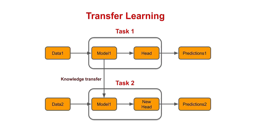
Also If you know about Transfer Learning then you might wonder why not instead of using a pretext task, we instead use transfer learning. Now that could work but there are a lot of times when the problem we’re trying to solve is a lot different than the tasks that existing models were trained on and so in those cases transfer learning doesn’t work as efficiently with limited labeled data.
I should also mention that although self-supervised learning has been successfully used in language-based tasks, it’s still in the adoption and development stage in Computer vision tasks. This is because, unlike text, it’s really hard to predict uncertainty in images, the output is not discrete and there are countless possibilities meaning there is not just one right answer. To learn more about these challenges, watch Yan Lecun’s ICLR presentation on self-supervised learning.
2 years back, Google published the SimCLR network in which they demonstrated an excellent self-supervised learning framework for image data. I would strongly recommend reading this excellent blog post in order to learn more on this topic. There are some very intuitive findings in this article that I can’t cover here.
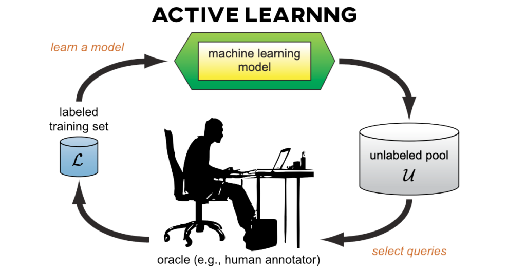
Besides Weak Supervision techniques, there are a few other methods like Transfer Learning and Active Learning. All of the techniques aim to partially or completely automate or reduce the data labeling or annotation process.
And this is a very active area of research these days, weak supervision techniques are closing the performance gap between them and supervised techniques. In the coming years, I expect to see wide adoption of Weak supervision and other similar techniques where manual data labeling is either no longer required or just minimally involved.
In Fact here’s what Yan LeCun, one of the pioneers of modern AI says:
“If artificial intelligence is a cake, self-supervised learning is the bulk of the cake,” “The next revolution in AI will not be supervised, nor purely reinforced”
Alright now let’s talk about Applied Fields of AI, AI industries, applications, and also let’s recap and summarize the entire field of AI and along with some very common issues.
So, here’s the thing … You might have read or heard these phrases.
Branches of AI, sub-branches of AI, Fields of AI, Subfields of AI, Domains of AI, or Subdomains of AI, Applications of AI, Industries of AI, AI paradigms.
Sometimes these phrases are accompanied by words like Applied AI Branches or Major AI Branches etc. And here’s the issue, I’ve seen numerous blog posts and people that used these phrases interchangeably. And I might be slightly guilty of that too. But the thing is, there is no strong consensus on what is major, applied branches, or sub Fields of AI. It’s a huge clutter of terminology out there.
In Fact, I actually googled some of these phrases and clicked to see images. But believe me, it was an abomination, to say the least.
I mean the way people had done categorization of AI Branches was an absolute mess. I mean seriously, the way people had mixed up AI applications with AI industries with AI branches …. it was just chaos… I’m not lying when I say I got a headache watching those graphs.
So here’s what I’m gonna do! I’m going to try to draw an abstract overview of the complete field of AI along with branches, subfields, applications, industries, and other things in this episode.
Complete Overview of AI Field
Now what I’m going to show you is just my personal overview and understanding of the AI field, and it can change as I continue to learn so I don’t expect everyone to agree with this categorization.
One final note, before we start: If you haven’t subscribed then please do so now. I’m planning to release more such tutorials and by subscribing you will get an email every time we release a tutorial.
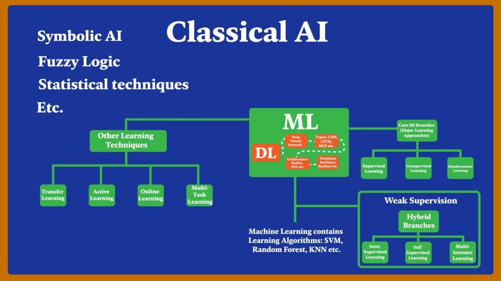
Alright, now let’s summarize the entire field of Artificial Intelligence. First off, We have Artificial Intelligence, I’m talking about Weak AI Or ANI (Artificial Narrow Intelligence), since we have made no real progress in AGI or ASI, we won’t be talking about that.
Inside AI, there is a subdomain called Machine Learning, now the area besides Machine learning is called Classical AI, this consists of rule-based Symbolic AI, Fuzzy logic, statistical techniques, and other classical methods. The domain of Machine learning itself consists of a set of algorithms that can learn from the data, these are SVM, Random Forest, KNN, etc.
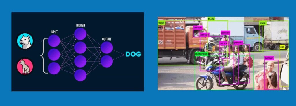
Inside machine learning is a subfield called Deep Learning, which is mostly concerned with Hierarchical learning algorithms called Deep Neural Networks. Now there are many types of Neural nets, e.g. Convolutional networks, LSTM, etc. And each type consists of many architectures which also have many variations.
Now machine learning (Including Deep learning) has 3 core branches or approaches, Supervised Learning, Unsupervised Learning, and Reinforcement Learning, we also have some hybrid branches which combine supervised and unsupervised methods. All of these can be categorized as Weak Supervision methods.
Now when studying machine learning, you might also come across learning approaches like Transfer Learning, Active Learning, and others. These are not broad fields but just learning techniques used in specific circumstances.
Alright now let’s take a look at some applied fields of AI, now there is no strong consensus but according to me there are 4 Applied Fields of AI; Computer Vision, Natural Language Processing, Speech, and Numerical Analysis. All 4 of these Applied fields use algorithms from either Classical AI, Machine Learning, or Deep Learning.
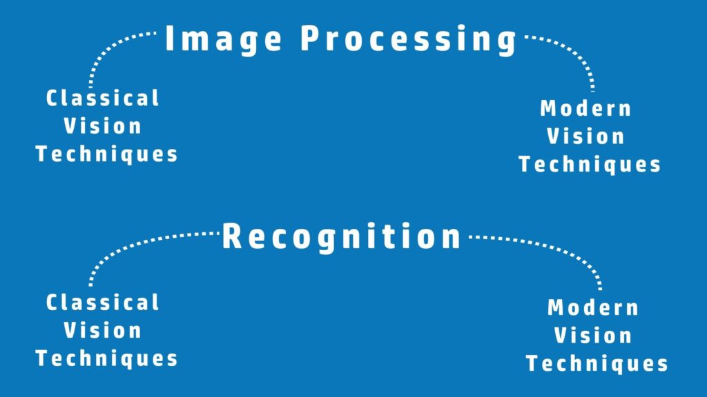
Let’s further look into these fields, Computer Vision can be split into 2 categories, Image Processing where we manipulate, process, or transform images. And Recognition, where we analyze content in images and make sense out of it. A lot of the time when people are talking about computer vision they are only referring to the recognition part.
Natural Language Processing can be broadly split into 2 parts; Natural Language Understanding; where you try to make sense of the textual data, interpret it, and understand its true meaning. And Natural Language Generation; where you try to generate meaningful text.
Btw the task of Language translation like in Google Translate uses both NLU & NLG
Speech can also be divided into 2 categories, Speech Recognition or Speech to text (STT); where you try to build systems that can understand speech and correctly predict the right text for it, and Speech Generation or text-to-speech (TTS); where you try to build systems able to generate realistic human-like speech.
And Finally Numerical Analytics; where you analyze numerical data to either gain meaningful insights or do predictive modeling, meaning you train models to learn from data and make useful predictions based on it.
Now I’m calling this numerical analytics but you can also call this Data Analytics or Data Science. I avoided the word “data” because Image, Text, and Speech are also data types.
And if you think about it, even data types like images, and text are converted to numbers at the end but, right now I’m defining numerical analytics as the field that analyzes numerical data other than these three data types.
Now since I work in Computer Vision, let me expand the computer vision field a bit.
So both of these categories (Image Processing and Recognition) can be further split into two types; Classical vision techniques and Modern vision techniques.
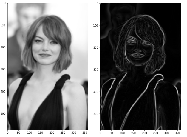
The only difference between the two types is that modern vision techniques use only Deep Learning based methods whereas Classical vision does not. So for example, Classical Image Processing can be things like image resizing, converting an image to grayscale, Canny edge detection, etc.
And Modern Image Processing can be things like Image Colorization via deep learning etc.
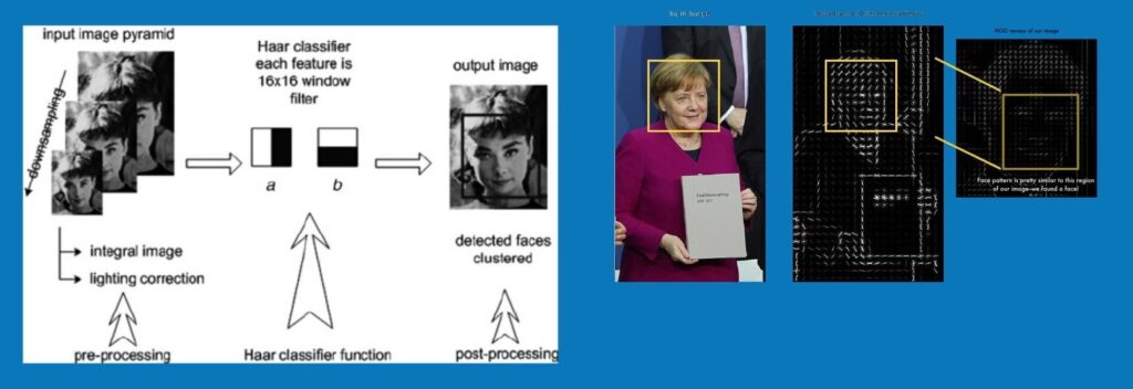
Classical Recognition can be things like: Face Detection with Haar cascades, and Histogram based Object detection.
And Modern Recognition can be things like Image Classification, Object Detection using neural networks, etc.
So these were Applied Fields of AI, Alright now let’s take a look at some Applied SubFields of AI. I’m defining Applied subfields as those fields that are built around certain specialized topics of any of the 4 applied fields I’ve mentioned.
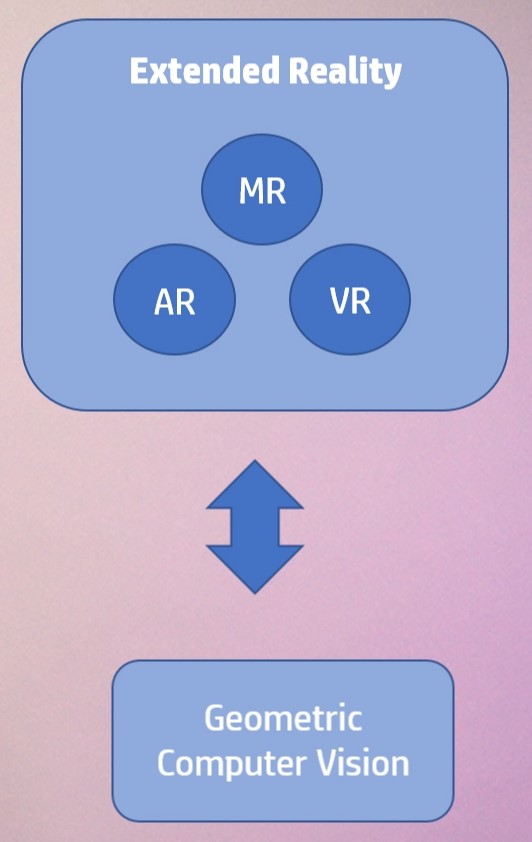
For example, Extended Reality is an applied subfield of AI built around a particular set of computer vision algorithms. It consists of Virtual Reality;
Augmented Reality;
and Mixed Reality;
You can even consider Extended Reality as a subdomain of Computer Vision. It’s worth mentioning that most of the computer vision techniques used in Extended reality itself fall in another domain of Computer Vision called Geometric Computer Vision, these algorithms deal with geometric relations between the 3D world and its projection into a 2D image.
There are many applied AI Subfields, another example of this would be Expert Systems which is an AI system that emulates the decision-making ability of a human expert.
So consider a Medical Diagnostic app that can take pictures of your skin and then a computer vision algorithm evaluates the picture to determine if you have any skin diseases.
Now, this system is performing a task that a dermatologist (skin expert) does, so it’s an example of an Expert system.
Rule-based Expert Systems became really popular in the 1980s and were considered a major feat in AI. These systems had two parts, a knowledge base, (A database containing all the facts provided by a human expert) and an inference engine that used the knowledge base and the observations from the user to give out results.
Although these types of expert systems are still used today, they have serious limitations. Now the example of the Expert system I just gave is from the Healthcare Industry and Expert systems can be found in other industries too.
Speaking of industries, let’s talk about AI applications used in industries. So these days AI is used in almost any industry you can think of, some popular categories are Automotive, Finance, Healthcare, Robotics, and others.
Within each Industry, you will find AI applications like self-driving cars, fraud detection, etc. All these applications are using methods & techniques from one of the 4 Applied AI Fields.
There are many applications that fail in multiple industries, for example, a humanoid robot built for amusement will fall in robotics and the entertainment industry. While the Self Driving car technologies fall into the transportation and automotive industry.
Also, an industry may split into subcategories. For example, Digital Media can be split into social media, streaming media, and other niche industries. By the way, most media sites use Recommendation Systems, which is yet another applied AI subdomain.
Join My Course Computer Vision For Building Cutting Edge Applications Course
The only course out there that goes beyond basic AI Applications and teaches you how to create next-level apps that utilize physics, deep learning, classical image processing, hand and body gestures. Don’t miss your chance to level up and take your career to new heights
You’ll Learn about:
Creating GUI interfaces for python AI scripts.
Creating .exe DL applications
Using a Physics library in Python & integrating it with AI
Advance Image Processing Skills
Advance Gesture Recognition with Mediapipe
Task Automation with AI & CV
Training an SVM machine Learning Model.
Creating & Cleaning an ML dataset from scratch.
Training DL models & how to use CNN’s & LSTMS.
Creating 10 Advance AI/CV Applications
& More
Whether you’re a seasoned AI professional or someone just looking to start out in AI, this is the course that will teach you, how to Architect & Build complex, real world and thrilling AI ap
Alright, so this was a high-level overview of the complete field of AI. Not everyone would agree with this categorization, but this categorization is necessary when you’re deciding which area of AI to focus on and how all the fields are connected to each other, and personally, I think this is one of the simplest and most intuitive abstract overviews of the AI field that you’ll find out there. Obviously, It was not meant to cover everything, but a high-level overview of the field.
This Concludes the 4th and final part of our Artificial Intelligence – 4 levels Explanation series. If you enjoyed this episode of computer vision for everyone then do subscribe to the Bleed AI YouTube channel and share it with your colleagues. Thank you.
Hire Us
Let our team of expert engineers and managers build your next big project using Bleeding Edge AI Tools & Technologies
Vehicle detection has been a challenging part of building intelligent traffic management systems. Such systems are critical for addressing the ever-increasing number of vehicles on road networks that cannot keep up with the pace of increasing traffic. Today many methods that deal with this problem use either traditional computer vision or complex deep learning models.
Popular computer vision techniques include vehicle detection using optical flow, but in this tutorial, we are going to perform vehicle detection using another traditional computer vision technique that utilizes background subtraction and contour detection to detect vehicles. This means you won’t have to spend hundreds of hours in data collection or annotation for building deep learning models, which can be tedious, to say the least. Not to mention, the computation power required to train the models.
This post is the fourth and final part of our Contour Detection 101 series. All 4 posts in the series are titled as:
Vehicle Detection with OpenCV using Contours + Background Subtraction (This Post)
So if you are new to the series and unfamiliar with contour detection, make sure you check them out!
In part 1 of the series, we learned the basics, how to detect and draw the contours, in part 2 we learned to do some contour manipulations and in the third part, we analyzed the detected contours for their properties to perform tasks like object detection. Combining these techniques with background subtraction will enable us to build a useful application that detects vehicles on a road. And not just that but you can use the same principles that you learn in this tutorial to create other motion detection applications.
So let’s dive into how vehicle detection with background subtraction works.
Import the Libraries
Let’s First start by importing the libraries.
import cv2
import numpy as np
import matplotlib.pyplot as plt
%matplotlib inline
Background subtraction is a simple yet effective technique to extract objects from an image/video. Consider a highway on which cars are moving, and you want to extract each car. One easy way can be that you take a picture of the highway with the cars (called foreground image) and you also have an image saved in which the highway does not contain any cars (background image) so you subtract the background image from the foreground to get the segmented mask of the cars and then use that mask to extract the cars.
But in many cases you don’t have a clear background image, an example of this can be a highway that is always busy, or maybe a walking destination that is always crowded. So in those cases, you can subtract the background by other means, for example, in the case of a video you can detect the movement of the object, so the objects which move can be foreground and the other part that remain static can be the background.
Several algorithms have been invented for this purpose. OpenCV has implemented a few such algorithms which are very easy to use. Let’s see one of them.
history (optional) – It is the length of the history. Its default value is 500.
varThreshold (optional) – It is the threshold on the squared distance between the pixel and the model to decide whether a pixel is well described by the background model. It does not affect the background update and its default value is 16.
detectShadows (optional) – It is a boolean that determines whether the algorithm will detect and mark shadows or not. It marks shadows in gray color. Its default value is True. It decreases the speed a bit, so if you do not need this feature, set the parameter to false.
Returns:
object – It is the MOG2 Background Subtractor.
# load a video
cap = cv2.VideoCapture('media/videos/vtest.avi')

# you can optionally work on the live web cam
# cap = cv2.VideoCapture(0)

# create the background object, you can choose to detect shadows or not (if True they will be shown as gray)
backgroundobject = cv2.createBackgroundSubtractorMOG2( history = 2, detectShadows = True )

while(1):
    ret, frame = cap.read()
    if not ret:
        break

    # apply the background object on each frame
    fgmask = backgroundobject.apply(frame)

    # also extracting the real detected foreground part of the image (optional)
    real_part = cv2.bitwise_and(frame,frame,mask=fgmask)

    # making fgmask 3 channeled so it can be stacked with others
    fgmask_3 = cv2.cvtColor(fgmask, cv2.COLOR_GRAY2BGR)

    # Stack all three frames and show the image
    stacked = np.hstack((fgmask_3,frame,real_part))
    cv2.imshow('All three',cv2.resize(stacked,None,fx=0.65,fy=0.65))

    k = cv2.waitKey(30) &  0xff
    if k == 27:
        break

cap.release()
cv2.destroyAllWindows()
Output:
The second frame is the original video, on the left we have the background subtraction result with shadows, while on the right we have the foreground part produced using the background subtraction mask.
Creating the Vehicle Detection Application
Alright once we have our background subtraction method ready, we can build our final application!
Here’s the breakdown of the steps we need to perform the complete background Subtraction based contour detection.
1) Start by loading the video using the function cv2.VideoCapture() and create a background subtractor object using the function cv2.createBackgroundSubtractorMOG2().
3) Next, we will apply thresholding on the mask using the function cv2.threshold() to get rid of shadows and then perform Erosion and Dilation to improve the mask further using the functions cv2.erode() and cv2.dilate().
4) Then we will use the function cv2.findContours() to detect the contours on the mask image and convert the contour coordinates into bounding box coordinates for each car in the frame using the function cv2.boundingRect(). We will also check the area of the contour using cv2.contourArea() to make sure it is greater than a threshold for a car contour.
5) After that we will use the functions cv2.rectangle() and cv2.putText() to draw and label the bounding boxes on each frame and extract the foreground part of the video with the help of the segmented mask using the function cv2.bitwise_and().
# load a video
video = cv2.VideoCapture('media/videos/carsvid.wmv')

# You can set custom kernel size if you want.
kernel = None

# Initialize the background object.
backgroundObject = cv2.createBackgroundSubtractorMOG2(detectShadows = True)

while True:

    # Read a new frame.
    ret, frame = video.read()

    # Check if frame is not read correctly.
    if not ret:

        # Break the loop.

        break

    # Apply the background object on the frame to get the segmented mask.
    fgmask = backgroundObject.apply(frame)
    #initialMask = fgmask.copy()

    # Perform thresholding to get rid of the shadows.
    _, fgmask = cv2.threshold(fgmask, 250, 255, cv2.THRESH_BINARY)
    #noisymask = fgmask.copy()

    # Apply some morphological operations to make sure you have a good mask
    fgmask = cv2.erode(fgmask, kernel, iterations = 1)
    fgmask = cv2.dilate(fgmask, kernel, iterations = 2)

    # Detect contours in the frame.
    contours, _ = cv2.findContours(fgmask, cv2.RETR_EXTERNAL, cv2.CHAIN_APPROX_SIMPLE)

    # Create a copy of the frame to draw bounding boxes around the detected cars.
    frameCopy = frame.copy()

    # loop over each contour found in the frame.
    for cnt in contours:

        # Make sure the contour area is somewhat higher than some threshold to make sure its a car and not some noise.
        if cv2.contourArea(cnt) > 400:

            # Retrieve the bounding box coordinates from the contour.
            x, y, width, height = cv2.boundingRect(cnt)

            # Draw a bounding box around the car.
            cv2.rectangle(frameCopy, (x , y), (x + width, y + height),(0, 0, 255), 2)

            # Write Car Detected near the bounding box drawn.
            cv2.putText(frameCopy, 'Car Detected', (x, y-10), cv2.FONT_HERSHEY_SIMPLEX, 0.3, (0,255,0), 1, cv2.LINE_AA)

    # Extract the foreground from the frame using the segmented mask.
    foregroundPart = cv2.bitwise_and(frame, frame, mask=fgmask)

    # Stack the original frame, extracted foreground, and annotated frame.
    stacked = np.hstack((frame, foregroundPart, frameCopy))

    # Display the stacked image with an appropriate title.
    cv2.imshow('Original Frame, Extracted Foreground and Detected Cars', cv2.resize(stacked, None, fx=0.5, fy=0.5))
    #cv2.imshow('initial Mask', initialMask)
    #cv2.imshow('Noisy Mask', noisymask)
    #cv2.imshow('Clean Mask', fgmask)


    # Wait until a key is pressed.
    # Retreive the ASCII code of the key pressed
    k = cv2.waitKey(1) & 0xff

    # Check if 'q' key is pressed.
    if k == ord('q'):

        # Break the loop.
        break

# Release the VideoCapture Object.
video.release()

# Close the windows
cv2.destroyAllWindows()
Output:
This seems to have worked out well, that too without having to train large-scale Deep learning models!
There are many other background subtraction algorithms in OpenCV that you can use. Check out here and here for further details about them.
Summary
Vehicle Detection is a popular computer vision problem. This post explored how traditional machine vision tools can still be utilized to build applications that can effectively deal with modern vision challenges.
We used a popular background/foreground segmentation technique called background subtraction to isolate our regions of interest from the image.
We also saw how contour detection can prove to be useful when dealing with vision problems. The pre-processing and post-processing that can be used to filter out the noise in the detected contours.
Although these techniques can be robust, they are not as generalizable as Deep learning models so it’s important to put more focus on deployment conditions and possible variations when building vision applications with such techniques.
This post concludes the four-part series on contour detection. If you enjoyed this post and followed the rest of the series do let me know in the comments and you can also support me and the Bleed AI team on patreon here.
If you need 1 on 1 Coaching in AI/computer vision regarding your project, or your career then you reach out to mepersonally here
Hire Us
Let our team of expert engineers and managers build your next big project using Bleeding Edge AI Tools & Technologies
In last Week’s tutorial, we learned how to work with real-time pose detection and created a pose classification system. In this week’s tutorial, we’ll learn to play a popular game called “Subway Surfers”
Of Course, there’s more to it, this is an AI Blog after all.
We will actually be using our body pose to control the game, not keyboard controls, the entire application will work in real-time on your CPU, you don’t even need a depth camera or a Kinect, your webcam will suffice.
Excited yet, let’s get into it, but before that let me tell you a short story that motivated me to build this application today. It starts with me giving a lecture on the importance of physical fitness, I know … I know … how this sounds but just bear with me for a bit.
Hi All, Taha Awnar here, So here’s the thing. One of the best things I enjoyed in my early teenage years was having a fast metabolism due to my involvement in physical activities. I could eat whatever I wanted, not make a conscious effort in exercising and still stay fit.
But as I grew older, and started spending most of my time in front of a computer, I noticed that I was actually gaining weight. So no longer could I afford the luxury of binge unhealthy eating and skipping workouts.
Now I’m a bit of a foodie so although I could compromise a bit on how I eat, I still needed to cut weight some other way, so I quickly realized that unless I wanted to get obese, I needed to consciously make effort to workout.
That’s about when I joined a local gym in my area, and guess what? … it didn’t work out, ( or I didn’t work out … enough 🙁 ) So I quitted after a month.
So what was the reason ?.… Well, I could provide multiple excuses but to be honest, I was just lazy.
A few months later I joined the gym again and again I quitted after just 2 months.
Now I could have just quit completely but instead 8 months back I tried again, this time I even hired a trainer to keep me motivated, and as they say it, 3rd time’s a charm and luckily it was!
8 months in, I’m still at it. I did see results and lost a couple of kgs, although I haven’t reached my personal target so I’m still working towards it.
If you’re reading this post then you’re probably into computer science just like me and you most likely need to spend a lot of time in front of a PC and because of that, your physical and mental fitness must take a toll. And I seriously can’t stress enough how important it is that you take out a couple of hours each week to exercise.
I’m not a fitness guru but I can say working out has many key benefits:
Helps you shed excess weight, keeps you physically fit.
Gives you mental clarity and improves your work quality.
Lots of health benefits.
Helps you get a partner, if you’re still single like me … lol
Because of these reasons, even though I have an introverted personality, I consciously take out a couple of hours each week to go to the gym or the park for running.
But here’s the thing, sometimes I wonder why can’t I combine what I do (working on a PC) with some activity so I could … you know hit 2 birds with one stone.
This thought led me to create this post today, so what I did was I created a vision application that allows me to control a very popular game called Subway Surfers via my body movement by utilizing real-time pose detection.
And so In this tutorial, I’ll show you how to create this application that controls the Subway Surfers game using body gestures and movements so that you can also exercise, code, and have fun at the same time.
How will this Work?
So this game is about a character running from a policeman dodging different hurdles by jumping, crouching, and moving left and right. So we will need to worry about four controls that are normally controlled using a keyboard.
Up arrow key to make the character jump
Down arrow key to make the character crouch
Left arrow key to move the character to left
Right arrow key to move the character to right.
Using the Pyautogui library, we will automatically trigger the required keypress events, depending upon the body movement of the person that we’ll capture using Mediapipe’s Pose Detection model.
I want the game’s character to:
Jump whenever the person controlling the character jumps.
Crouch whenever the person controlling the character crouches.
Move left whenever the person controlling the character moves to the left side of the screen.
Move right whenever the person controlling the character moves to the right on the screen.
You can also use the techniques you’ll learn in this tutorial to control any other game. The simpler the game, the easier it will be to control. I have actually published two tutorials about game control via body gestures.
Alright now that we have discussed the basic mechanisms for creating this application, let me walk you through the exact step-by-step process I used to create this.
Outline
Step 1: Perform Pose Detection
Step 2: Control Starting Mechanism
Step 3: Control Horizontal Movements
Step 4: Control Vertical Movements
Step 5: Control Keyboard and Mouse with PyautoGUI
Step 6: Build the Final Application
Alright, let’s get started.
Download Code
[optin-monster slug=”fosdrzvuquq2gad1pccq”]
Import the Libraries
We will start by importing the required libraries.
import cv2
import pyautogui
from time import time
from math import hypot
import mediapipe as mp
import matplotlib.pyplot as plt
Initialize the Pose Detection Model
After that we will need to initialize the mp.solutions.pose class and then call the mp.solutions.pose.Pose() function with appropriate arguments and also initialize mp.solutions.drawing_utils class that is needed to visualize the landmarks after detection.
# Initialize mediapipe pose class.
mp_pose = mp.solutions.pose

# Setup the Pose function for images.
pose_image = mp_pose.Pose(static_image_mode=True, min_detection_confidence=0.5, model_complexity=1)

# Setup the Pose function for videos.
pose_video = mp_pose.Pose(static_image_mode=False, model_complexity=1, min_detection_confidence=0.7,
                          min_tracking_confidence=0.7)

# Initialize mediapipe drawing class.
mp_drawing = mp.solutions.drawing_utils
Step 1: Perform Pose Detection
To implement the game control mechanisms, we will need the current pose info of the person controlling the game, as our intention is to control the character with the movement of the person in the frame. We want the game’s character to move left, right, jump and crouch with the identical movements of the person.
So we will create a function detectPose() that will take an image as input and perform pose detection on the person in the image using the mediapipe’s pose detection solution to get thirty-three 3D landmarks on the body and the function will display the results or return them depending upon the passed arguments.
This function is quite similar to the one we had created in the previous post. The only difference is that we are not plotting the pose landmarks in 3D and we are passing a few more optional arguments to the function mp.solutions.drawing_utils.draw_landmarks() to specify the drawing style.
You probably do not want to lose control of the game’s character whenever some other person comes into the frame (and starts controlling the character), so that annoying scenario is already taken care of, as the solution we are using only detects the landmarks of the most prominent person in the image.
So you do not need to worry about losing control as long as you are the most prominent person in the frame as it will automatically ignore the people in the background.
def detectPose(image, pose, draw=False, display=False):
    '''
    This function performs the pose detection on the most prominent person in an image.
    Args:
        image:   The input image with a prominent person whose pose landmarks needs to be detected.
        pose:    The pose function required to perform the pose detection.
        draw:    A boolean value that is if set to true the function draw pose landmarks on the output image.
        display: A boolean value that is if set to true the function displays the original input image, and the
                 resultant image and returns nothing.
    Returns:
        output_image: The input image with the detected pose landmarks drawn if it was specified.
        results:      The output of the pose landmarks detection on the input image.
    '''

    # Create a copy of the input image.
    output_image = image.copy()

    # Convert the image from BGR into RGB format.
    imageRGB = cv2.cvtColor(image, cv2.COLOR_BGR2RGB)

    # Perform the Pose Detection.
    results = pose.process(imageRGB)

    # Check if any landmarks are detected and are specified to be drawn.
    if results.pose_landmarks and draw:

        # Draw Pose Landmarks on the output image.
        mp_drawing.draw_landmarks(image=output_image, landmark_list=results.pose_landmarks,
                                  connections=mp_pose.POSE_CONNECTIONS,
                                  landmark_drawing_spec=mp_drawing.DrawingSpec(color=(255,255,255),
                                                                               thickness=3, circle_radius=3),
                                  connection_drawing_spec=mp_drawing.DrawingSpec(color=(49,125,237),
                                                                               thickness=2, circle_radius=2))

    # Check if the original input image and the resultant image are specified to be displayed.
    if display:

        # Display the original input image and the resultant image.
        plt.figure(figsize=[22,22])
        plt.subplot(121);plt.imshow(image[:,:,::-1]);plt.title("Original Image");plt.axis('off');
        plt.subplot(122);plt.imshow(output_image[:,:,::-1]);plt.title("Output Image");plt.axis('off');

    # Otherwise
    else:

        # Return the output image and the results of pose landmarks detection.
        return output_image, results
Now we will test the function detectPose() created above to perform pose detection on a sample image and display the results.
# Read a sample image and perform pose landmarks detection on it.
IMG_PATH = 'media/sample.jpg'
image = cv2.imread(IMG_PATH)
detectPose(image, pose_image, draw=True, display=True
It worked pretty well! if you want you can test the function on other images too by just changing the value of the variable IMG_PATH in the cell above, it will work fine as long as there is a prominent person in the image.
Step 2: Control Starting Mechanism
In this step, we will implement the game starting mechanism, what we want is to start the game whenever the most prominent person in the image/frame joins his both hands together. So we will create a function checkHandsJoined() that will check whether the hands of the person in an image are joined or not.
The function checkHandsJoined() will take in the results of the pose detection returned by the function detectPose() and will use the LEFT_WRIST and RIGHT_WRIST landmarks coordinates from the list of thirty-three landmarks, to calculate the euclidean distance between the hands of the person.
And then utilize an appropriate threshold value to compare with and check whether the hands of the person in the image/frame are joined or not and will display or return the results depending upon the passed arguments.
def checkHandsJoined(image, results, draw=False, display=False):
    '''
    This function checks whether the hands of the person are joined or not in an image.
    Args:
        image:   The input image with a prominent person whose hands status (joined or not) needs to be classified.
        results: The output of the pose landmarks detection on the input image.
        draw:    A boolean value that is if set to true the function writes the hands status & distance on the output image.
        display: A boolean value that is if set to true the function displays the resultant image and returns nothing.
    Returns:
        output_image: The same input image but with the classified hands status written, if it was specified.
        hand_status:  The classified status of the hands whether they are joined or not.
    '''

    # Get the height and width of the input image.
    height, width, _ = image.shape

    # Create a copy of the input image to write the hands status label on.
    output_image = image.copy()

    # Get the left wrist landmark x and y coordinates.
    left_wrist_landmark = (results.pose_landmarks.landmark[mp_pose.PoseLandmark.LEFT_WRIST].x * width,
                          results.pose_landmarks.landmark[mp_pose.PoseLandmark.LEFT_WRIST].y * height)

    # Get the right wrist landmark x and y coordinates.
    right_wrist_landmark = (results.pose_landmarks.landmark[mp_pose.PoseLandmark.RIGHT_WRIST].x * width,
                           results.pose_landmarks.landmark[mp_pose.PoseLandmark.RIGHT_WRIST].y * height)

    # Calculate the euclidean distance between the left and right wrist.
    euclidean_distance = int(hypot(left_wrist_landmark[0] - right_wrist_landmark[0],
                                   left_wrist_landmark[1] - right_wrist_landmark[1]))

    # Compare the distance between the wrists with a appropriate threshold to check if both hands are joined.
    if euclidean_distance < 130:

        # Set the hands status to joined.
        hand_status = 'Hands Joined'

        # Set the color value to green.
        color = (0, 255, 0)

    # Otherwise.
    else:

        # Set the hands status to not joined.
        hand_status = 'Hands Not Joined'

        # Set the color value to red.
        color = (0, 0, 255)

    # Check if the Hands Joined status and hands distance are specified to be written on the output image.
    if draw:

        # Write the classified hands status on the image.
        cv2.putText(output_image, hand_status, (10, 30), cv2.FONT_HERSHEY_PLAIN, 2, color, 3)

        # Write the the distance between the wrists on the image.
        cv2.putText(output_image, f'Distance: {euclidean_distance}', (10, 70),
                    cv2.FONT_HERSHEY_PLAIN, 2, color, 3)

    # Check if the output image is specified to be displayed.
    if display:

        # Display the output image.
        plt.figure(figsize=[10,10])
        plt.imshow(output_image[:,:,::-1]);plt.title("Output Image");plt.axis('off');

    # Otherwise
    else:

        # Return the output image and the classified hands status indicating whether the hands are joined or not.
        return output_image, hand_status
Now we will test the function checkHandsJoined() created above on a real-time webcam feed to check whether it is working as we had expected or not.
# Initialize the VideoCapture object to read from the webcam.
camera_video = cv2.VideoCapture(1)
camera_video.set(3,1280)
camera_video.set(4,960)

# Create named window for resizing purposes.
cv2.namedWindow('Hands Joined?', cv2.WINDOW_NORMAL)

# Iterate until the webcam is accessed successfully.
while camera_video.isOpened():

    # Read a frame.
    ok, frame = camera_video.read()

    # Check if frame is not read properly then continue to the next iteration to read the next frame.
    if not ok:
        continue

    # Flip the frame horizontally for natural (selfie-view) visualization.
    frame = cv2.flip(frame, 1)

    # Get the height and width of the frame of the webcam video.
    frame_height, frame_width, _ = frame.shape

    # Perform the pose detection on the frame.
    frame, results = detectPose(frame, pose_video, draw=True)

    # Check if the pose landmarks in the frame are detected.
    if results.pose_landmarks:

        # Check if the left and right hands are joined.
        frame, _ = checkHandsJoined(frame, results, draw=True)

    # Display the frame.
    cv2.imshow('Hands Joined?', frame)

    # Wait for 1ms. If a key is pressed, retreive the ASCII code of the key.
    k = cv2.waitKey(1) & 0xFF

    # Check if 'ESC' is pressed and break the loop.
    if(k == 27):
        break

# Release the VideoCapture Object and close the windows.
camera_video.release()
cv2.destroyAllWindows()
Output Video:
Woah! I am stunned, the pose detection solution is best known for its speed which is reflecting in the results as the distance and the hands status are updating very fast and are also highly accurate.
Step 3: Control Horizontal Movements
Now comes the implementation of the left and right movements control mechanism of the game’s character, what we want to do is to make the game’s character move left and right with the horizontal movements of the person in the image/frame.
So we will create a function checkLeftRight() that will take in the pose detection results returned by the function detectPose() and will use the x-coordinates of the RIGHT_SHOULDER and LEFT_SHOULDER landmarks to determine the horizontal position (Left, Right or Center) in the frame after comparing the landmarks with the x-coordinate of the center of the image.
The function will visualize or return the resultant image and the horizontal position of the person depending upon the passed arguments.
def checkLeftRight(image, results, draw=False, display=False):
    '''
    This function finds the horizontal position (left, center, right) of the person in an image.
    Args:
        image:   The input image with a prominent person whose the horizontal position needs to be found.
        results: The output of the pose landmarks detection on the input image.
        draw:    A boolean value that is if set to true the function writes the horizontal position on the output image.
        display: A boolean value that is if set to true the function displays the resultant image and returns nothing.
    Returns:
        output_image:         The same input image but with the horizontal position written, if it was specified.
        horizontal_position:  The horizontal position (left, center, right) of the person in the input image.
    '''

    # Declare a variable to store the horizontal position (left, center, right) of the person.
    horizontal_position = None

    # Get the height and width of the image.
    height, width, _ = image.shape

    # Create a copy of the input image to write the horizontal position on.
    output_image = image.copy()

    # Retreive the x-coordinate of the left shoulder landmark.
    left_x = int(results.pose_landmarks.landmark[mp_pose.PoseLandmark.RIGHT_SHOULDER].x * width)

    # Retreive the x-corrdinate of the right shoulder landmark.
    right_x = int(results.pose_landmarks.landmark[mp_pose.PoseLandmark.LEFT_SHOULDER].x * width)

    # Check if the person is at left that is when both shoulder landmarks x-corrdinates
    # are less than or equal to the x-corrdinate of the center of the image.
    if (right_x <= width//2 and left_x <= width//2):

        # Set the person's position to left.
        horizontal_position = 'Left'

    # Check if the person is at right that is when both shoulder landmarks x-corrdinates
    # are greater than or equal to the x-corrdinate of the center of the image.
    elif (right_x >= width//2 and left_x >= width//2):

        # Set the person's position to right.
        horizontal_position = 'Right'

    # Check if the person is at center that is when right shoulder landmark x-corrdinate is greater than or equal to
    # and left shoulder landmark x-corrdinate is less than or equal to the x-corrdinate of the center of the image.
    elif (right_x >= width//2 and left_x <= width//2):

        # Set the person's position to center.
        horizontal_position = 'Center'

    # Check if the person's horizontal position and a line at the center of the image is specified to be drawn.
    if draw:

        # Write the horizontal position of the person on the image.
        cv2.putText(output_image, horizontal_position, (5, height - 10), cv2.FONT_HERSHEY_PLAIN, 2, (255, 255, 255), 3)

        # Draw a line at the center of the image.
        cv2.line(output_image, (width//2, 0), (width//2, height), (255, 255, 255), 2)

    # Check if the output image is specified to be displayed.
    if display:

        # Display the output image.
        plt.figure(figsize=[10,10])
        plt.imshow(output_image[:,:,::-1]);plt.title("Output Image");plt.axis('off');

    # Otherwise
    else:

        # Return the output image and the person's horizontal position.
        return output_image, horizontal_position
Now we will test the function checkLeftRight() created above on a real-time webcam feed and will visualize the results updating in real-time with the horizontal movements.
# Initialize the VideoCapture object to read from the webcam.
camera_video = cv2.VideoCapture(1)
camera_video.set(3,1280)
camera_video.set(4,960)

# Create named window for resizing purposes.
cv2.namedWindow('Horizontal Movements', cv2.WINDOW_NORMAL)

# Iterate until the webcam is accessed successfully.
while camera_video.isOpened():

    # Read a frame.
    ok, frame = camera_video.read()

    # Check if frame is not read properly then continue to the next iteration to read the next frame.
    if not ok:
        continue

    # Flip the frame horizontally for natural (selfie-view) visualization.
    frame = cv2.flip(frame, 1)

    # Get the height and width of the frame of the webcam video.
    frame_height, frame_width, _ = frame.shape

    # Perform the pose detection on the frame.
    frame, results = detectPose(frame, pose_video, draw=True)

    # Check if the pose landmarks in the frame are detected.
    if results.pose_landmarks:

        # Check the horizontal position of the person in the frame.
        frame, _ = checkLeftRight(frame, results, draw=True)

    # Display the frame.
    cv2.imshow('Horizontal Movements', frame)

    # Wait for 1ms. If a a key is pressed, retreive the ASCII code of the key.
    k = cv2.waitKey(1) & 0xFF

    # Check if 'ESC' is pressed and break the loop.
    if(k == 27):
        break

# Release the VideoCapture Object and close the windows.
camera_video.release()
cv2.destroyAllWindows()
Output Video:
Cool! the speed and accuracy of this model never fail to impress me.
Step 4: Control Vertical Movements
In this one, we will implement the jump and crouch control mechanism of the game’s character, what we want is to make the game’s character jump and crouch whenever the person in the image/frame jumps and crouches.
So we will create a function checkJumpCrouch() that will check whether the posture of the person in an image is Jumping, Crouching or Standing by utilizing the results of pose detection by the function detectPose().
The function checkJumpCrouch() will retrieve the RIGHT_SHOULDER and LEFT_SHOULDER landmarks from the list to calculate the y-coordinate of the midpoint of both shoulders and will determine the posture of the person by doing a comparison with an appropriate threshold value.
The threshold (MID_Y) will be the approximate y-coordinate of the midpoint of both shoulders of the person while in standing posture. It will be calculated before starting the game in the Step 6: Build the Final Application and will be passed to the function checkJumpCrouch().
But the issue with this approach is that the midpoint of both shoulders of the person while in standing posture will not always be exactly the same as it will vary when the person will move closer or further to the camera.
To tackle this issue we will add and subtract a margin to the threshold to get an upper and lower bound as shown in the image below.
def checkJumpCrouch(image, results, MID_Y=250, draw=False, display=False):
    '''
    This function checks the posture (Jumping, Crouching or Standing) of the person in an image.
    Args:
        image:   The input image with a prominent person whose the posture needs to be checked.
        results: The output of the pose landmarks detection on the input image.
        MID_Y:   The intial center y-coordinate of both shoulders landmarks of the person recorded during starting
                 the game. This will give the idea of the person's height when he is standing straight.
        draw:    A boolean value that is if set to true the function writes the posture on the output image.
        display: A boolean value that is if set to true the function displays the resultant image and returns nothing.
    Returns:
        output_image: The input image with the person's posture written, if it was specified.
        posture:      The posture (Jumping, Crouching or Standing) of the person in an image.
    '''

    # Get the height and width of the image.
    height, width, _ = image.shape

    # Create a copy of the input image to write the posture label on.
    output_image = image.copy()

    # Retreive the y-coordinate of the left shoulder landmark.
    left_y = int(results.pose_landmarks.landmark[mp_pose.PoseLandmark.RIGHT_SHOULDER].y * height)

    # Retreive the y-coordinate of the right shoulder landmark.
    right_y = int(results.pose_landmarks.landmark[mp_pose.PoseLandmark.LEFT_SHOULDER].y * height)

    # Calculate the y-coordinate of the mid-point of both shoulders.
    actual_mid_y = abs(right_y + left_y) // 2

    # Calculate the upper and lower bounds of the threshold.
    lower_bound = MID_Y-15
    upper_bound = MID_Y+100

    # Check if the person has jumped that is when the y-coordinate of the mid-point
    # of both shoulders is less than the lower bound.
    if (actual_mid_y < lower_bound):

        # Set the posture to jumping.
        posture = 'Jumping'

    # Check if the person has crouched that is when the y-coordinate of the mid-point
    # of both shoulders is greater than the upper bound.
    elif (actual_mid_y > upper_bound):

        # Set the posture to crouching.
        posture = 'Crouching'

    # Otherwise the person is standing and the y-coordinate of the mid-point
    # of both shoulders is between the upper and lower bounds.
    else:

        # Set the posture to Standing straight.
        posture = 'Standing'

    # Check if the posture and a horizontal line at the threshold is specified to be drawn.
    if draw:

        # Write the posture of the person on the image.
        cv2.putText(output_image, posture, (5, height - 50), cv2.FONT_HERSHEY_PLAIN, 2, (255, 255, 255), 3)

        # Draw a line at the intial center y-coordinate of the person (threshold).
        cv2.line(output_image, (0, MID_Y),(width, MID_Y),(255, 255, 255), 2)

    # Check if the output image is specified to be displayed.
    if display:

        # Display the output image.
        plt.figure(figsize=[10,10])
        plt.imshow(output_image[:,:,::-1]);plt.title("Output Image");plt.axis('off');

    # Otherwise
    else:

        # Return the output image and posture indicating whether the person is standing straight or has jumped, or crouched.
        return output_image, posture
Now we will test the function checkJumpCrouch() created above on the real-time webcam feed and will visualize the resultant frames. For testing purposes, we will be using a default value of the threshold, that if you want you can tune manually set according to your height.
# Initialize the VideoCapture object to read from the webcam.
camera_video = cv2.VideoCapture(1)
camera_video.set(3,1280)
camera_video.set(4,960)

# Create named window for resizing purposes.
cv2.namedWindow('Verticial Movements', cv2.WINDOW_NORMAL)

# Iterate until the webcam is accessed successfully.
while camera_video.isOpened():

    # Read a frame.
    ok, frame = camera_video.read()

    # Check if frame is not read properly then continue to the next iteration to read the next frame.
    if not ok:
        continue

    # Flip the frame horizontally for natural (selfie-view) visualization.
    frame = cv2.flip(frame, 1)

    # Get the height and width of the frame of the webcam video.
    frame_height, frame_width, _ = frame.shape

    # Perform the pose detection on the frame.
    frame, results = detectPose(frame, pose_video, draw=True)

    # Check if the pose landmarks in the frame are detected.
    if results.pose_landmarks:

        # Check the posture (jumping, crouching or standing) of the person in the frame.
        frame, _ = checkJumpCrouch(frame, results, draw=True)

    # Display the frame.
    cv2.imshow('Verticial Movements', frame)

    # Wait for 1ms. If a a key is pressed, retreive the ASCII code of the key.
    k = cv2.waitKey(1) & 0xFF

    # Check if 'ESC' is pressed and break the loop.
    if(k == 27):
        break

# Release the VideoCapture Object and close the windows.
camera_video.release()
cv2.destroyAllWindows()
Output Video:
Great! when I lower my shoulders at a certain range from the horizontal line (threshold), the results are Crouching, and the results are Standing, whenever my shoulders are near the horizontal line (i.e., between the upper and lower bounds), and when my shoulders are at a certain range above the horizontal line, the results are Jumping.
Step 5: Control Keyboard and Mouse with PyautoGUI
The Subway Surfers character wouldn’t be able to move left, right, jump or crouch unless we provide it the required keyboard inputs. Now that we have the functions checkHandsJoined(), checkLeftRight() and checkJumpCrouch(), we need to figure out a way to trigger the required keyboard keypress events, depending upon the output of the functions created above.
This is where the PyAutoGUI API shines. It allows you to easily control the mouse and keyboard event through scripts. To get an idea of PyAutoGUI’s capabilities, you can check this video in which a bot is playing the game Sushi Go Round.
To run the cells in this step, it is not recommended to use the keyboard keys (Shift + Enter) as the cells with keypress events will behave differently when the events will be combined with the keys Shift and Enter. You can either use the menubar (Cell>>Run Cell) or the toolbar (▶️Run) to run the cells.
Now let’s see how simple it is to trigger the up arrow keypress event using pyautogui.
# Press the up key.
pyautogui.press(keys='up')
Similarly, we can trigger the down arrow or any other keypress event by replacing the argument with that key name (the argument should be a string). You can click here to see the list of valid arguments.
# Press the down key.
pyautogui.press(keys='down')
To press multiple keys, we can pass a list of strings (key names) to the pyautogui.press() function.
# Press the up (4 times) and down (1 time) key.
pyautogui.press(keys=['up', 'up', 'up', 'up', 'down'])
Or to press the same key multiple times, we can pass a value (number of times we want to press the key) to the argument presses in the pyautogui.press() function.
# Press the down key 4 times.
pyautogui.press(keys='down', presses=4)
This function presses the key(s) down and then releases up the key(s) automatically. We can also control this keypress event and key release event individually by using the functions:
pyautogui.keyDown(key): Presses and holds down the specified key.
pyautogui.keyUp(key): Releases up the specified key.
So with the help of these functions, keys can be pressed for a longer period. Like in the cell below we will hold down the shift key and press the enter key (two times) to run the two cells below this one and then we will release the shift key.
# Hold down the shift key.
pyautogui.keyDown(key='shift')

# Press the enter key two times.
pyautogui.press(keys='enter', presses=2)

# Release the shift key.
pyautogui.keyUp(key='shift')
# This cell will run automatically due to keypress events in the previous cell.
print('Hello!')
# This cell will also run automatically due to those keypress events.
print('Happy Learning!')
Now we will hold down the shift key and press the tab key and then we will release the shift key. This will switch the tab of your browser so make sure to have multiple tabs before running the cell below.
# Hold down the shift key.
pyautogui.keyDown(key='ctrl')

# Press the tab key.
pyautogui.press(keys='tab')

# Release the shift key.
pyautogui.keyUp(key='ctrl')
To trigger the mouse key press events, we can use pyautogui.click() function and to specify the mouse button that we want to press, we can pass the values left, middle, or right to the argument button.
# Press the mouse right button. It will open up the menu.
pyautogui.click(button='right')
We can also move the mouse cursor to a specific position on the screen by specifying the x and y-coordinate values to the arguments x and y respectively.
# Move to 1300, 800, then click the right mouse button
pyautogui.click(x=1300, y=800, button='right')
Step 6: Build the Final Application
In the final step, we will have to combine all the components to build the final application.
We will use the outputs of the functions created above checkHandsJoined() (to start the game), checkLeftRight() (control horizontal movements) and checkJumpCrouch() (control vertical movements) to trigger the relevant keyboard and mouse events and control the game’s character with our body movements.
Now we will run the cell below and click here to play the game in our browser using our body gestures and movements.
# Initialize the VideoCapture object to read from the webcam.
camera_video = cv2.VideoCapture(0)
camera_video.set(3,1280)
camera_video.set(4,960)

# Create named window for resizing purposes.
cv2.namedWindow('Subway Surfers with Pose Detection', cv2.WINDOW_NORMAL)

# Initialize a variable to store the time of the previous frame.
time1 = 0

# Initialize a variable to store the state of the game (started or not).
game_started = False

# Initialize a variable to store the index of the current horizontal position of the person.
# At Start the character is at center so the index is 1 and it can move left (value 0) and right (value 2).
x_pos_index = 1

# Initialize a variable to store the index of the current vertical posture of the person.
# At Start the person is standing so the index is 1 and he can crouch (value 0) and jump (value 2).
y_pos_index = 1

# Declate a variable to store the intial y-coordinate of the mid-point of both shoulders of the person.
MID_Y = None

# Initialize a counter to store count of the number of consecutive frames with person's hands joined.
counter = 0

# Initialize the number of consecutive frames on which we want to check if person hands joined before starting the game.
num_of_frames = 10

# Iterate until the webcam is accessed successfully.
while camera_video.isOpened():

    # Read a frame.
    ok, frame = camera_video.read()

    # Check if frame is not read properly then continue to the next iteration to read the next frame.
    if not ok:
        continue

    # Flip the frame horizontally for natural (selfie-view) visualization.
    frame = cv2.flip(frame, 1)

    # Get the height and width of the frame of the webcam video.
    frame_height, frame_width, _ = frame.shape

    # Perform the pose detection on the frame.
    frame, results = detectPose(frame, pose_video, draw=game_started)

    # Check if the pose landmarks in the frame are detected.
    if results.pose_landmarks:

        # Check if the game has started
        if game_started:

            # Commands to control the horizontal movements of the character.
            #--------------------------------------------------------------------------------------------------------------

            # Get horizontal position of the person in the frame.
            frame, horizontal_position = checkLeftRight(frame, results, draw=True)

            # Check if the person has moved to left from center or to center from right.
            if (horizontal_position=='Left' and x_pos_index!=0) or (horizontal_position=='Center' and x_pos_index==2):

                # Press the left arrow key.
                pyautogui.press('left')

                # Update the horizontal position index of the character.
                x_pos_index -= 1

            # Check if the person has moved to Right from center or to center from left.
            elif (horizontal_position=='Right' and x_pos_index!=2) or (horizontal_position=='Center' and x_pos_index==0):

                # Press the right arrow key.
                pyautogui.press('right')

                # Update the horizontal position index of the character.
                x_pos_index += 1

            #--------------------------------------------------------------------------------------------------------------

        # Otherwise if the game has not started
        else:

            # Write the text representing the way to start the game on the frame.
            cv2.putText(frame, 'JOIN BOTH HANDS TO START THE GAME.', (5, frame_height - 10), cv2.FONT_HERSHEY_PLAIN,
                        2, (0, 255, 0), 3)

        # Command to Start or resume the game.
        #------------------------------------------------------------------------------------------------------------------

        # Check if the left and right hands are joined.
        if checkHandsJoined(frame, results)[1] == 'Hands Joined':

            # Increment the count of consecutive frames with +ve condition.
            counter += 1

            # Check if the counter is equal to the required number of consecutive frames.
            if counter == num_of_frames:

                # Command to Start the game first time.
                #----------------------------------------------------------------------------------------------------------

                # Check if the game has not started yet.
                if not(game_started):

                    # Update the value of the variable that stores the game state.
                    game_started = True

                    # Retreive the y-coordinate of the left shoulder landmark.
                    left_y = int(results.pose_landmarks.landmark[mp_pose.PoseLandmark.RIGHT_SHOULDER].y * frame_height)

                    # Retreive the y-coordinate of the right shoulder landmark.
                    right_y = int(results.pose_landmarks.landmark[mp_pose.PoseLandmark.LEFT_SHOULDER].y * frame_height)

                    # Calculate the intial y-coordinate of the mid-point of both shoulders of the person.
                    MID_Y = abs(right_y + left_y) // 2

                    # Move to 1300, 800, then click the left mouse button to start the game.
                    pyautogui.click(x=1300, y=800, button='left')

                #----------------------------------------------------------------------------------------------------------

                # Command to resume the game after death of the character.
                #----------------------------------------------------------------------------------------------------------

                # Otherwise if the game has started.
                else:

                    # Press the space key.
                    pyautogui.press('space')

                #----------------------------------------------------------------------------------------------------------

                # Update the counter value to zero.
                counter = 0

        # Otherwise if the left and right hands are not joined.
        else:

            # Update the counter value to zero.
            counter = 0

        #------------------------------------------------------------------------------------------------------------------

        # Commands to control the vertical movements of the character.
        #------------------------------------------------------------------------------------------------------------------

        # Check if the intial y-coordinate of the mid-point of both shoulders of the person has a value.
        if MID_Y:

            # Get posture (jumping, crouching or standing) of the person in the frame.
            frame, posture = checkJumpCrouch(frame, results, MID_Y, draw=True)

            # Check if the person has jumped.
            if posture == 'Jumping' and y_pos_index == 1:

                # Press the up arrow key
                pyautogui.press('up')

                # Update the veritcal position index of  the character.
                y_pos_index += 1

            # Check if the person has crouched.
            elif posture == 'Crouching' and y_pos_index == 1:

                # Press the down arrow key
                pyautogui.press('down')

                # Update the veritcal position index of the character.
                y_pos_index -= 1

            # Check if the person has stood.
            elif posture == 'Standing' and y_pos_index   != 1:

                # Update the veritcal position index of the character.
                y_pos_index = 1

        #------------------------------------------------------------------------------------------------------------------


    # Otherwise if the pose landmarks in the frame are not detected.
    else:

        # Update the counter value to zero.
        counter = 0

    # Calculate the frames updates in one second
    #----------------------------------------------------------------------------------------------------------------------

    # Set the time for this frame to the current time.
    time2 = time()

    # Check if the difference between the previous and this frame time > 0 to avoid division by zero.
    if (time2 - time1) > 0:

        # Calculate the number of frames per second.
        frames_per_second = 1.0 / (time2 - time1)

        # Write the calculated number of frames per second on the frame.
        cv2.putText(frame, 'FPS: {}'.format(int(frames_per_second)), (10, 30),cv2.FONT_HERSHEY_PLAIN, 2, (0, 255, 0), 3)

    # Update the previous frame time to this frame time.
    # As this frame will become previous frame in next iteration.
    time1 = time2

    #----------------------------------------------------------------------------------------------------------------------

    # Display the frame.
    cv2.imshow('Subway Surfers with Pose Detection', frame)

    # Wait for 1ms. If a a key is pressed, retreive the ASCII code of the key.
    k = cv2.waitKey(1) & 0xFF

    # Check if 'ESC' is pressed and break the loop.
    if(k == 27):
        break

# Release the VideoCapture Object and close the windows.
camera_video.release()
cv2.destroyAllWindows()
Output Video:
While building big applications like this one, I always divide the application into smaller components and then, in the end, integrate all those components to make the final application.
This makes it really easy to learn and understand how everything comes together to build up the full application.
Join My Course Computer Vision For Building Cutting Edge Applications Course
The only course out there that goes beyond basic AI Applications and teaches you how to create next-level apps that utilize physics, deep learning, classical image processing, hand and body gestures. Don’t miss your chance to level up and take your career to new heights
You’ll Learn about:
Creating GUI interfaces for python AI scripts.
Creating .exe DL applications
Using a Physics library in Python & integrating it with AI
Advance Image Processing Skills
Advance Gesture Recognition with Mediapipe
Task Automation with AI & CV
Training an SVM machine Learning Model.
Creating & Cleaning an ML dataset from scratch.
Training DL models & how to use CNN’s & LSTMS.
Creating 10 Advance AI/CV Applications
& More
Whether you’re a seasoned AI professional or someone just looking to start out in AI, this is the course that will teach you, how to Architect & Build complex, real world and thrilling AI applications
In this tutorial, we learned to perform pose detection on the most prominent person in the frame/image, to get thirty-three 3D landmarks, and then use those landmarks to extract useful info about the body movements (horizontal position i.e., left, center or right and posture i.e. jumping, standing or crouching) of the person and then use that info to control a simple game.
Another thing we have learned is how to automatically trigger the mouse and keyboard events programmatically using the Pyautogui library.
Now one drawback of controlling the game with body movements is that the game becomes much harder compared to controlling it via keyboard presses.
But our aim to make the exercise fun and learn to control Human-Computer Interaction (HCI) based games using AI is achieved. Now if you want, you can extend this application further to control a much more complex application.
You can reach out to me personally for a 1 on 1 consultation session in AI/computer vision regarding your project. Our talented team of vision engineers will help you every step of the way. Get on a call with me directlyhere.
Ready to seriously dive into State of the Art AI & Computer Vision? Then Sign up for these premium Courses by Bleed AI
In this tutorial, we’ll learn how to do real-time 3D hands landmarks detection using the Mediapipe library in python. After that, we’ll learn to perform hands type classification (i.e. is it a left or right hand) and then draw the bounding boxes around the hands by retrieving the required coordinates from the detected landmarks.
Below are the results on a few sample images, and this will work on real-time camera feed or recorded videos as well.
And last but not the least, we will also create a customized landmarks annotation of the hands utilizing the depth (distance from the camera) of the hands, as Mediapipe’s solution provides three-dimensional landmarks.
The annotation provided by Mediapipe allows users to annotate the images and videos with a single line of code but it does not utilize the depth and draws fixed-sized lines and circles on the hands.
But in our customized annotation, the thickness of the lines (connections) and circles (landmarks) for each hand will vary in real-time by using the depth of each hand, with the decrease in the distance from the camera (depth), the size of the annotation increases.
The motivation behind this was that the size of the hand in the image/frame increases when the hand is moved closer to the camera, so using a fixed size annotation for a hand that varies in size was hard to digest for me. You can see the comparison of Mediapipe’s annotation and our customized annotation below.
The code for all this is very easy and is explained in the simplest manner possible.
Now before diving further, you can go and watch the youtube tutorial for the detailed explanation, although this blog post alone can also serve the purpose.
In this one, we will learn to localize twenty-one key landmarks on hand(s) e.g. wrist, thumb and fingertips, etc. See the image below:
It is an important and popular pre-processing task in many vision applications as it allows to localize and recognize the shape and motion of hands that opens up the door to the future by making a ton of applications feasible like:
Augmented Reality Applications that overlay Digital Content and Information over Reality like a Virtual Painter.
Sign Language Recognition.
Hand Gesture Controlled Drones and Robots or any other Physical Appliances.
Using landmark detection is also a great way to interact with any Human-Computer Interaction (HCI) based system as the human hand is capable of making multiple gestures without much effort.
Some other types of keypoint detection problems are facial landmark detection, pose detection, etc.
I have already made a tutorial on pose detection and will explain facial landmark detection in an upcoming tutorial.
Part 1 (b): Mediapipe’s Hands Landmarks Detection Implementation
Here’s a brief introduction to Mediapipe;
“Mediapipe is a cross-platform/open-source tool that allows you to run a variety of machine learning models in real-time. It’s designed primarily for facilitating the use of ML in streaming media & It was built by Google”
All the models in Mediapipe have state-of-the-art performance and are highly optimized as well and are used in a lot of well-known products out there.
It provides a robust solution capable of predicting twenty-one 3D landmarks on a hand in real-time with high accuracy and speed as well, even on low-end devices i.e. phones, laptops, etc., which makes it stand out from the other solutions out there.
Now you may be thinking what makes it so fast?
Actually, they have combined a computationally costly object detector with an object tracker that requires a lot less processing. So for the videos, a tracker is used instead of invoking the object detector at every frame which makes this solution so fast and brilliant.
The detector is only invoked as needed, that is in the very first frame or when the tracker loses track of any of the hands. The detector localizes the hand in the image/frame and outputs the bounding box coordinates around the hand.
Then the region of interest (ROI) is cropped from the image/frame using the bounding box coordinates and after that, the cropped image/frame is used by the hand landmark model to predict the landmarks within the ROI.
The palm detector is used, as detecting hands is a comparatively more complex task than the palm or fist (i.e., rigid objects). Palms require square bounding boxes which reduces the number of anchors (predefined bounding boxes of a certain height and width). Also as palms are smaller objects, which reduces the possibility of self-occlusion (hidden by themselves), like handshakes. Comparatively, hands lack easily distinguishable patterns and are often occluded.
The image below shows the twenty-one hand landmarks, that this solution detects, along with their indexes.
They manually annotated around 30K real-world images with 3D coordinates by using images depth maps and also rendered a high-quality synthetic hand model over various backgrounds and then mapped the model with different backgrounds to the corresponding 3D coordinates.
So they kind of automated the whole annotation process. The image below contains the aligned hands cropped images and the rendered synthetic hand images with ground truth annotation.
Alright now we have learned the required basic theory and implementation details, let’s dive into the code.
Download Code:
[optin-monster slug=”ko5ox1sveedosrhdesgq”]
Import the Libraries
We will start by importing the required libraries.
import cv2
import numpy as np
from time import time
import mediapipe as mp
import matplotlib.pyplot as plt
Part 2: Using Hands Landmarks Detection on images and videos
Initialize the Hands Landmarks Detection Model
To use the Mediapipe’s hands solution, we first have to initialize the hands class using the mp.solutions.hands syntax and then we will have to call the function mp.solutions.hands.Hands() with the arguments explained below:
static_image_mode – It is a boolean value that is if set to False, the solution treats the input images as a video stream. It will try to detect hands in the first input images, and upon a successful detection further localizes the hand landmarks. In subsequent images, once all max_num_hands hands are detected and the corresponding hand landmarks are localized, it simply tracks those landmarks without invoking another detection until it loses track of any of the hands. This reduces latency and is ideal for processing video frames. If set to True, hand detection runs on every input image, ideal for processing a batch of static, possibly unrelated, images. Its default value is False.
max_num_hands – It is the maximum number of hands to detect. Its default value is 2.
min_detection_confidence – It is the minimum detection confidence ([0.0, 1.0]) required to consider the palm-detection model’s prediction correct. Its default value is 0.5 which means that all the detections with prediction confidence less than 50% are ignored by default.
min_tracking_confidence – It is the minimum tracking confidence ([0.0, 1.0]) required to consider the landmark-tracking model’s tracked hands landmarks valid. If the confidence is less than this argument value then the detector is invoked again in the next frame/image, so increasing its value increases the robustness, but also increases the latency. Its default value is 0.5.
Then we will also need to initialize the mp.solutions.drawing_utils class that is very useful to visualize the landmarks on the images/frames.
# Initialize the mediapipe hands class.
mp_hands = mp.solutions.hands

# Set up the Hands function.
hands = mp_hands.Hands(static_image_mode=True, max_num_hands=2, min_detection_confidence=0.3)

# Initialize the mediapipe drawing class.
mp_drawing = mp.solutions.drawing_utils
Read an Image
Now we will use the function cv2.imread() to read a sample image and then display it using the matplotlib library.
# Read an image from the specified path.
sample_img = cv2.imread('media/sample.jpg')

# Specify a size of the figure.
plt.figure(figsize = [10, 10])

# Display the sample image, also convert BGR to RGB for display.
plt.title("Sample Image");plt.axis('off');plt.imshow(sample_img[:,:,::-1]);plt.show()
Perform Hands Landmarks Detection
Now we will pass the image to the hand’s landmarks detection machine learning pipeline by using the function mp.solutions.hands.Hands().process(). But first, we will have to convert the image from BGR to RGB format using the function cv2.cvtColor() as OpenCV reads images in BGR format and the ml pipeline expects the input images to be in RGB color format.
The machine learning pipeline outputs a list of twenty-one landmarks of the prominent hands in the image. Each landmark has:
x – It is the landmark x-coordinate normalized to [0.0, 1.0] by the image width.
y: It is the landmark y-coordinate normalized to [0.0, 1.0] by the image height.
z: It is the landmark z-coordinate normalized to roughly the same scale as x. It represents the landmark depth with the wrist being the origin, so the smaller the value the closer the landmark is to the camera.
To get more intuition, we will display the first two landmarks of each hand, the ml pipeline outputs an object that has an attribute multi_hand_landmarks that contains the found landmarks coordinates of each hand as an element of a list.
Note:The z-coordinate is just the relative distance of the landmark from the wrist, and this distance increases and decreases depending upon the distance from the camera so that is why it represents the depth of each landmark point.
# Perform hands landmarks detection after converting the image into RGB format.
results = hands.process(cv2.cvtColor(sample_img, cv2.COLOR_BGR2RGB))

# Check if landmarks are found.
if results.multi_hand_landmarks:

    # Iterate over the found hands.
    for hand_no, hand_landmarks in enumerate(results.multi_hand_landmarks):

        print(f'HAND NUMBER: {hand_no+1}')
        print('-----------------------')

        # Iterate two times as we only want to display first two landmarks of each hand.
        for i in range(2):

            # Display the found normalized landmarks.
            print(f'{mp_hands.HandLandmark(i).name}:')
            print(f'{hand_landmarks.landmark[mp_hands.HandLandmark(i).value]}')
As you can see that the landmarks are normalized to specific scales, so now we will convert them back to their original scale by using the width and height of the sample image and display them.
# Retrieve the height and width of the sample image.
image_height, image_width, _ = sample_img.shape

# Check if landmarks are found.
if results.multi_hand_landmarks:

    # Iterate over the found hands.
    for hand_no, hand_landmarks in enumerate(results.multi_hand_landmarks):

        print(f'HAND NUMBER: {hand_no+1}')
        print('-----------------------')

        # Iterate two times as we only want to display first two landmark of each hand.
        for i in range(2):

            # Display the found landmarks after converting them into their original scale.
            print(f'{mp_hands.HandLandmark(i).name}:')
            print(f'x: {hand_landmarks.landmark[mp_hands.HandLandmark(i).value].x * image_width}')
            print(f'y: {hand_landmarks.landmark[mp_hands.HandLandmark(i).value].y * image_height}')
            print(f'z: {hand_landmarks.landmark[mp_hands.HandLandmark(i).value].z * image_width}\n')
Now we will draw the detected landmarks on a copy of the sample image using the function mp.solutions.drawing_utils.draw_landmarks() from the class mp.solutions.drawing_utils, we had initialized earlier and will display the resultant image.
# Create a copy of the sample image to draw landmarks on.
img_copy = sample_img.copy()

# Check if landmarks are found.
if results.multi_hand_landmarks:

    # Iterate over the found hands.
    for hand_no, hand_landmarks in enumerate(results.multi_hand_landmarks):

        # Draw the hand landmarks on the copy of the sample image.
        mp_drawing.draw_landmarks(image = img_copy, landmark_list = hand_landmarks,
                                  connections = mp_hands.HAND_CONNECTIONS)

    # Specify a size of the figure.
    fig = plt.figure(figsize = [10, 10])

    # Display the resultant image with the landmarks drawn, also convert BGR to RGB for display.
    plt.title("Resultant Image");plt.axis('off');plt.imshow(img_copy[:,:,::-1]);plt.show()
Part 3: Hands Classification (i.e., Left or Right)
Create a Hands Landmarks Detection Function
Now we will put all this together to create a function that will perform hands landmarks detection on an image and will visualize the resultant image along with the original image or return the resultant image along with the output of the model depending upon the passed arguments.
def detectHandsLandmarks(image, hands, display = True):
    '''
    This function performs hands landmarks detection on an image.
    Args:
        image:   The input image with prominent hand(s) whose landmarks needs to be detected.
        hands:   The hands function required to perform the hands landmarks detection.
        display: A boolean value that is if set to true the function displays the original input image, and the output
                 image with hands landmarks drawn and returns nothing.
    Returns:
        output_image: The input image with the detected hands landmarks drawn.
        results: The output of the hands landmarks detection on the input image.
    '''

    # Create a copy of the input image to draw landmarks on.
    output_image = image.copy()

    # Convert the image from BGR into RGB format.
    imgRGB = cv2.cvtColor(image, cv2.COLOR_BGR2RGB)

    # Perform the Hands Landmarks Detection.
    results = hands.process(imgRGB)

    # Check if landmarks are found.
    if results.multi_hand_landmarks:

        # Iterate over the found hands.
        for hand_landmarks in results.multi_hand_landmarks:

            # Draw the hand landmarks on the copy of the input image.
            mp_drawing.draw_landmarks(image = output_image, landmark_list = hand_landmarks,
                                  connections = mp_hands.HAND_CONNECTIONS)

    # Check if the original input image and the output image are specified to be displayed.
    if display:

        # Display the original input image and the output image.
        plt.figure(figsize=[15,15])
        plt.subplot(121);plt.imshow(image[:,:,::-1]);plt.title("Original Image");plt.axis('off');
        plt.subplot(122);plt.imshow(output_image[:,:,::-1]);plt.title("Output");plt.axis('off');

    # Otherwise
    else:

        # Return the output image and results of hands landmarks detection.
        return output_image, results
Now we will utilize the function created above to perform hands landmarks detection on a few sample images and display the results.
# Read another sample image and perform hands landmarks detection on it.
image = cv2.imread('media/sample1.jpg')
detectHandsLandmarks(image, hands, display=True)
# Read another sample image and perform hands landmarks detection on it.
image = cv2.imread('media/sample2.jpg')
detectHandsLandmarks(image, hands, display=True)
# Read another sample image and perform hands landmarks detection on it.
image = cv2.imread('media/sample3.jpg')
detectHandsLandmarks(image, hands, display=True)
Hands Landmarks Detection on Real-Time Webcam Feed
The results on the images were excellent, but now the real test begins, we will try the function on a real-time webcam feed. We will also calculate and display the number of frames being updated in one second to get an idea of whether this solution can work in real-time on a CPU or not. As that is the only thing that differentiates it from the other solutions out there.
# Setup Hands function for video.
hands_video = mp_hands.Hands(static_image_mode=False, max_num_hands=2,
                             min_detection_confidence=0.7, min_tracking_confidence=0.4)

# Initialize the VideoCapture object to read from the webcam.
camera_video = cv2.VideoCapture(1)
camera_video.set(3,1280)
camera_video.set(4,960)

# Create named window for resizing purposes.
cv2.namedWindow('Hands Landmarks Detection', cv2.WINDOW_NORMAL)

# Initialize a variable to store the time of the previous frame.
time1 = 0

# Iterate until the webcam is accessed successfully.
while camera_video.isOpened():

    # Read a frame.
    ok, frame = camera_video.read()

    # Check if frame is not read properly then continue to the next iteration to read the next frame.
    if not ok:
        continue

    # Flip the frame horizontally for natural (selfie-view) visualization.
    frame = cv2.flip(frame, 1)

    # Perform Hands landmarks detection.
    frame, _ = detectHandsLandmarks(frame, hands_video, display=False)

    # Set the time for this frame to the current time.
    time2 = time()

    # Check if the difference between the previous and this frame time > 0 to avoid division by zero.
    if (time2 - time1) > 0:

        # Calculate the number of frames per second.
        frames_per_second = 1.0 / (time2 - time1)

        # Write the calculated number of frames per second on the frame.
        cv2.putText(frame, 'FPS: {}'.format(int(frames_per_second)), (10, 30),cv2.FONT_HERSHEY_PLAIN, 2, (0, 255, 0), 3)

    # Update the previous frame time to this frame time.
    # As this frame will become previous frame in next iteration.
    time1 = time2

    # Display the frame.
    cv2.imshow('Hands Landmarks Detection', frame)

    # Wait for 1ms. If a a key is pressed, retreive the ASCII code of the key.
    k = cv2.waitKey(1) & 0xFF

    # Check if 'ESC' is pressed and break the loop.
    if(k == 27):
        break

# Release the VideoCapture Object and close the windows.
camera_video.release()
cv2.destroyAllWindows()
Output
Woah! that was impressive not only it was fast but the results were quite accurate too.
Create a Hand Type Classification Function
Now we will create a function that will perform hands type classification (i.e. is it a left or right hand). The output (object) by the hand’s landmarks detector model contains another attribute multi_handedness that contains a score (probability of the predicted label being correct) and label (either "Left" or "Right") for each detected hand.
While determining the label, it is assumed that the input image is mirrored (i.e., flipped horizontally). So we had already performed classification during the hand’s landmarks detection, and now we only need to access the information stored in the attribute multi_handedness.
def getHandType(image, results, draw=True, display = True):
    '''
    This function performs hands type (left or right) classification on hands.
    Args:
        image:   The image of the hands that needs to be classified, with the hands landmarks detection already performed.
        results: The output of the hands landmarks detection performed on the image in which hands types needs
                 to be classified.
        draw:    A boolean value that is if set to true the function writes the hand type label on the output image.
        display: A boolean value that is if set to true the function displays the output image and returns nothing.
    Returns:
        output_image: The image of the hands with the classified hand type label written if it was specified.
        hands_status: A dictionary containing classification info of both hands.
    '''

    # Create a copy of the input image to write hand type label on.
    output_image = image.copy()

    # Initialize a dictionary to store the classification info of both hands.
    hands_status = {'Right': False, 'Left': False, 'Right_index' : None, 'Left_index': None}

    # Iterate over the found hands in the image.
    for hand_index, hand_info in enumerate(results.multi_handedness):

        # Retrieve the label of the found hand.
        hand_type = hand_info.classification[0].label

        # Update the status of the found hand.
        hands_status[hand_type] = True

        # Update the index of the found hand.
        hands_status[hand_type + '_index'] = hand_index

        # Check if the hand type label is specified to be written.
        if draw:

            # Write the hand type on the output image.
            cv2.putText(output_image, hand_type + ' Hand Detected', (10, (hand_index+1) * 30),cv2.FONT_HERSHEY_PLAIN,
                        2, (0,255,0), 2)

    # Check if the output image is specified to be displayed.
    if display:

        # Display the output image.
        plt.figure(figsize=[10,10])
        plt.imshow(output_image[:,:,::-1]);plt.title("Output Image");plt.axis('off');

    # Otherwise
    else:

        # Return the output image and the hands status dictionary that contains classification info.
        return output_image, hands_status
Now we will utilize the function created above to perform hand type classification on a few sample images and display the results.
# Read a sample image with one hand and perform hand type classification on it after flipping it horizontally.
image = cv2.imread('media/sample5.jpg')
flipped_image = cv2.flip(image, 1)
_, results = detectHandsLandmarks(flipped_image, hands, display=False)
if results.multi_hand_landmarks:
    getHandType(image, results)
# Read a sample image with one hand and perform hand type classification on it after flipping it horizontally.
image = cv2.imread('media/sample6.jpg')
flipped_image = cv2.flip(image, 1)
_, results = detectHandsLandmarks(flipped_image, hands, display=False)
if results.multi_hand_landmarks:
    getHandType(image, results)
# Read a sample image with one hand and perform hand type classification on it after flipping it horizontally.
image = cv2.imread('media/sample7.jpg')
flipped_image = cv2.flip(image, 1)
_, results = detectHandsLandmarks(flipped_image, hands, display=False)
if results.multi_hand_landmarks:
    getHandType(image, results)
Cool! it worked perfectly on each of the sample images.
Part 4 (a): Draw Bounding Boxes around the Hands
Create a Function to Draw Bounding Boxes
Now we will create a function that will draw bounding boxes around the hands and write their classified types near them. We will first convert the normalized landmarks back to their original scale by using the width and height of the image. We will then get the bounding box coordinates ((x1,y1), (x2, y2)) for each hand.
Top Left Coordinate:
x1 – the smallest x-coordinate in the list of the found landmarks of the hand.
y1 – the smallest y-coordinate in the list of the found landmarks of the hand.
Bottom Right Coordinate:
x2 – the largest x-coordinate in the list of the found landmarks of the hand.
y2 – the largest y-coordinate in the list of the found landmarks of the hand.
Then we will draw the bounding boxes around the hands using the found coordinates and the specified padding and write the classified types of each hand near them using the bounding box coordinates. And after that, we will either display the resultant image or return it depending upon the passed arguments.
def drawBoundingBoxes(image, results, hand_status, padd_amount = 10, draw=True, display=True):
    '''
    This function draws bounding boxes around the hands and write their classified types near them.
    Args:
        image:       The image of the hands on which the bounding boxes around the hands needs to be drawn and the
                     classified hands types labels needs to be written.
        results:     The output of the hands landmarks detection performed on the image on which the bounding boxes needs
                     to be drawn.
        hand_status: The dictionary containing the classification info of both hands.
        padd_amount: The value that specifies the space inside the bounding box between the hand and the box's borders.
        draw:        A boolean value that is if set to true the function draws bounding boxes and write their classified
                     types on the output image.
        display:     A boolean value that is if set to true the function displays the output image and returns nothing.
    Returns:
        output_image:     The image of the hands with the bounding boxes drawn and hands classified types written if it
                          was specified.
        output_landmarks: The dictionary that stores both (left and right) hands landmarks as different elements.
    '''

    # Create a copy of the input image to draw bounding boxes on and write hands types labels.
    output_image = image.copy()

    # Initialize a dictionary to store both (left and right) hands landmarks as different elements.
    output_landmarks = {}

    # Get the height and width of the input image.
    height, width, _ = image.shape

    # Iterate over the found hands.
    for hand_index, hand_landmarks in enumerate(results.multi_hand_landmarks):

        # Initialize a list to store the detected landmarks of the hand.
        landmarks = []

        # Iterate over the detected landmarks of the hand.
        for landmark in hand_landmarks.landmark:

            # Append the landmark into the list.
            landmarks.append((int(landmark.x * width), int(landmark.y * height),
                                  (landmark.z * width)))

        # Get all the x-coordinate values from the found landmarks of the hand.
        x_coordinates = np.array(landmarks)[:,0]

        # Get all the y-coordinate values from the found landmarks of the hand.
        y_coordinates = np.array(landmarks)[:,1]

        # Get the bounding box coordinates for the hand with the specified padding.
        x1  = int(np.min(x_coordinates) - padd_amount)
        y1  = int(np.min(y_coordinates) - padd_amount)
        x2  = int(np.max(x_coordinates) + padd_amount)
        y2  = int(np.max(y_coordinates) + padd_amount)

        # Initialize a variable to store the label of the hand.
        label = "Unknown"

        # Check if the hand we are iterating upon is the right one.
        if hand_status['Right_index'] == hand_index:

            # Update the label and store the landmarks of the hand in the dictionary.
            label = 'Right Hand'
            output_landmarks['Right'] = landmarks

        # Check if the hand we are iterating upon is the left one.
        elif hand_status['Left_index'] == hand_index:

            # Update the label and store the landmarks of the hand in the dictionary.
            label = 'Left Hand'
            output_landmarks['Left'] = landmarks

        # Check if the bounding box and the classified label is specified to be written.
        if draw:

            # Draw the bounding box around the hand on the output image.
            cv2.rectangle(output_image, (x1, y1), (x2, y2), (155, 0, 255), 3, cv2.LINE_8)

            # Write the classified label of the hand below the bounding box drawn.
            cv2.putText(output_image, label, (x1, y2+25), cv2.FONT_HERSHEY_COMPLEX, 0.7, (20,255,155), 1, cv2.LINE_AA)

    # Check if the output image is specified to be displayed.
    if display:

        # Display the output image.
        plt.figure(figsize=[10,10])
        plt.imshow(output_image[:,:,::-1]);plt.title("Output Image");plt.axis('off');

    # Otherwise
    else:

        # Return the output image and the landmarks dictionary.
        return output_image, output_landmarks
Now we will utilize the function created above to perform hand type classification and draw bounding boxes around the hands on a real-time webcam feed.
# Initialize the VideoCapture object to read from the webcam.
camera_video = cv2.VideoCapture(1)

# Initialize a resizable window.
cv2.namedWindow('Hands Landmarks Detection', cv2.WINDOW_NORMAL)

# Iterate until the webcam is accessed successfully.
while camera_video.isOpened():

    # Read a frame.
    ok, frame = camera_video.read()

    # Check if frame is not read properly then continue to the next iteration to read the next frame.
    if not ok:
        continue

    # Flip the frame horizontally for natural (selfie-view) visualization.
    frame = cv2.flip(frame, 1)

    # Perform Hands landmarks detection.
    frame, results = detectHandsLandmarks(frame, hands_video, display=False)

    # Check if landmarks are found in the frame.
    if results.multi_hand_landmarks:

        # Perform hand(s) type (left or right) classification.
        _, hands_status = getHandType(frame.copy(), results, draw=False, display=False)

        # Draw bounding boxes around the detected hands and write their classified types near them.
        frame, _ = drawBoundingBoxes(frame, results, hands_status, display=False)

    # Display the frame.
    cv2.imshow('Hands Landmarks Detection', frame)

    # Wait for 1ms. If a a key is pressed, retreive the ASCII code of the key.
    k = cv2.waitKey(1) & 0xFF

    # Check if 'ESC' is pressed and break the loop.
    if(k == 27):
        break

# Release the VideoCapture Object and close the windows.
camera_video.release()
cv2.destroyAllWindows()
Output
Great! the classification, along with localization, works pretty accurately on a real-time webcam feed too.
Part 4 (b): Draw Bounding Boxes around the Hands
Create a Function to Draw Customized Landmarks Annotation
Now we will create a function that will draw customized landmarks of the hands. What we are doing differently, is that we are utilizing the depth (z-coordinate) values to increase and decrease the size of the lines and circles whereas Mediapipe’s annotation uses the fixed sizes. As we have learned that z-coordinate represents the landmark depth, so the smaller the value the closer the landmark is to the camera.
We are calculating the average depth of every landmark of a hand and with the decrease in the average depth of a hand, we are increasing the thickness of the annotation circles and the lines of that hand which means the closer the hand is to the camera bigger the annotation will be, to adjust the annotation size with the size of the hand.
def customLandmarksAnnotation(image, landmark_dict):
    '''
    This function draws customized landmarks annotation utilizing the z-coordinate (depth) values of the hands.
    Args:
        image:         The image of the hands on which customized landmarks annotation of the hands needs to be drawn.
        landmark_dict: The dictionary that stores the hand(s) landmarks as different elements with keys as hand
                       types(i.e., left and right).
    Returns:
        output_image: The image of the hands with the customized annotation drawn.
        depth:        A dictionary that contains the average depth of all landmarks of the hand(s) in the image.
    '''

    # Create a copy of the input image to draw annotation on.
    output_image = image.copy()

    # Initialize a dictionary to store the average depth of all landmarks of hand(s).
    depth = {}

    # Initialize a list with the arrays of indexes of the landmarks that will make the required
    # line segments to draw on the hand.
    segments = [np.arange(0,5), np.arange(5,9) , np.arange(9,13), np.arange(13, 17), np.arange(17, 21),
                np.arange(5,18,4), np.array([0,5]), np.array([0,17])]

    # Iterate over the landmarks dictionary.
    for hand_type, hand_landmarks in landmark_dict.items():

        # Get all the z-coordinates (depth) of the landmarks of the hand.
        depth_values = np.array(hand_landmarks)[:,-1]

        # Calculate the average depth of the hand.
        average_depth = int(sum(depth_values) / len(depth_values))

        # Get all the x-coordinates of the landmarks of the hand.
        x_values = np.array(hand_landmarks)[:,0]

        # Get all the y-coordinates of the landmarks of the hand.
        y_values = np.array(hand_landmarks)[:,1]

        # Initialize a list to store the arrays of x and y coordinates of the line segments for the hand.
        line_segments = []

        # Iterate over the arrays of indexes of the landmarks that will make the required line segments.
        for segment_indexes in segments:

            # Get an array of a line segment coordinates of the hand.
            line_segment = np.array([[int(x_values[index]), int(y_values[index])] for index in segment_indexes])

            # Append the line segment coordinates into the list.
            line_segments.append(line_segment)

        # Check if the average depth of the hand is less than 0.
        if average_depth < 0:

            # Set the thickness of the line segments of the hand accordingly to the average depth.
            line_thickness = int(np.ceil(0.1*abs(average_depth))) + 2

            # Set the thickness of the circles of the hand landmarks accordingly to the average depth.
            circle_thickness = int(np.ceil(0.1*abs(average_depth))) + 3

        # Otherwise.
        else:

            # Set the thickness of the line segments of the hand to 2 (i.e. the minimum thickness we are specifying).
            line_thickness = 2

            # Set the thickness of the circles to 3 (i.e. the minimum thickness)
            circle_thickness = 3

        # Draw the line segments on the hand.
        cv2.polylines(output_image, line_segments, False, (100,250,55), line_thickness)

        # Write the average depth of the hand on the output image.
        cv2.putText(output_image,'Depth: {}'.format(average_depth),(10,30), cv2.FONT_HERSHEY_COMPLEX, 1, (20,25,255), 1,
                    cv2.LINE_AA)

        # Iterate over the x and y coordinates of the hand landmarks.
        for x, y in zip(x_values, y_values):

            # Draw a circle on the x and y coordinate of the hand.
            cv2.circle(output_image,(int(x), int(y)), circle_thickness, (55,55,250), -1)

        # Store the calculated average depth in the dictionary.
        depth[hand_type] = average_depth

    # Return the output image and the average depth dictionary of the hand(s).
    return output_image, depth
Mediapipe’s Annotation vs Our Customized Annotation on Real-Time Webcam Feed
Now we will utilize the function created above to draw the customized annotation on a real-time webcam feed and stack it with the results of Mediapipe’s annotation to visualize the difference.
# Initialize the VideoCapture object to read from the webcam.
camera_video = cv2.VideoCapture(1)

# Initialize a resizable window.
cv2.namedWindow('Hands Landmarks Detection', cv2.WINDOW_NORMAL)

# Iterate until the webcam is accessed successfully.
while camera_video.isOpened():

    # Read a frame.
    ok, frame = camera_video.read()

    # Check if frame is not read properly then continue to the next iteration to read the next frame.
    if not ok:
        continue

    # Flip the frame horizontally for natural (selfie-view) visualization.
    frame = cv2.flip(frame, 1)

    # Perform Hands landmarks detection.
    annotated_frame, results = detectHandsLandmarks(frame, hands_video, display=False)

    # Check if landmarks are found in the frame.
    if results.multi_hand_landmarks:

        # Perform hand(s) type (left or right) classification.
        _, hands_status = getHandType(frame.copy(), results, draw=False, display=False)

        # Get the landmarks dictionary that stores each hand landmarks as different elements.
        frame, landmark_dict = drawBoundingBoxes(frame, results, hands_status, draw=False, display=False)

        # Draw customized landmarks annotation ultilizing the z-coordinate (depth) values of the hand(s).
        custom_ann_frame, _ = customLandmarksAnnotation(frame, landmark_dict)

        # Stack the frame annotated using mediapipe with the customized one.
        final_output = np.hstack((annotated_frame, custom_ann_frame))

    # Otherwise.
    else:

        # Stack the frame two time.
        final_output = np.hstack((frame, frame))

    # Display the stacked frame.
    cv2.imshow('Hands Landmarks Detection', final_output)

    # Wait for 1ms. If a a key is pressed, retreive the ASCII code of the key.
    k = cv2.waitKey(1) & 0xFF

    # Check if 'ESC' is pressed and break the loop.
    if(k == 27):
        break

# Release the VideoCapture Object and close the windows.
camera_video.release()
cv2.destroyAllWindows()
Output
As expected, the results were remarkable! The thickness of the annotation circles and the lines of each hand increased with the decrease in the distance, so the hack that Mediapipe uses to calculate the depth works pretty well and is also computationally very reasonable.
Join My Course Computer Vision For Building Cutting Edge Applications Course
The only course out there that goes beyond basic AI Applications and teaches you how to create next-level apps that utilize physics, deep learning, classical image processing, hand and body gestures. Don’t miss your chance to level up and take your career to new heights
You’ll Learn about:
Creating GUI interfaces for python AI scripts.
Creating .exe DL applications
Using a Physics library in Python & integrating it with AI
Advance Image Processing Skills
Advance Gesture Recognition with Mediapipe
Task Automation with AI & CV
Training an SVM machine Learning Model.
Creating & Cleaning an ML dataset from scratch.
Training DL models & how to use CNN’s & LSTMS.
Creating 10 Advance AI/CV Applications
& More
Whether you’re a seasoned AI professional or someone just looking to start out in AI, this is the course that will teach you, how to Architect & Build complex, real world and thrilling AI applications
In this tutorial, we have learned about a very popular and useful computer vision problem called hand landmarks detection. First, we covered what exactly this is, along with its applications, and then we moved to the implementation details that Mediapipe has used to provide the solution.
Also, we learned how it used a detection/tracker pipeline to provide the speed for which it stands out. After that, we performed 3D hands landmarks detection using Mediapipe’s solution on images and a real-time webcam feed.
Then we learned to classify hands as left or right and draw bounding boxes around them and after that, we learned to draw customized landmarks annotation utilizing the z-coordinate (depth) values of the hands.
Now a drawback of using this hand landmarks detection system is that you have to provide the maximum number of hands possible in the image/frame beforehand and the computationally expensive detector is invoked on every frame until the number of hands detection becomes equal to the provided maximum number of hands.
Another limitation is that the z-coordinate is just the relative distance of the landmark from the wrist, and that distance can also vary depending upon the posture of the hand i.e., whether the hand is closed or wide open. So it does not truly represent the depth, but still, it’s a great hack to calculate the depth from 2D images without using a depth camera.
You can reach out to me personally for a 1 on 1 consultation session in AI/computer vision regarding your project. Our talented team of vision engineers will help you every step of the way. Get on a call with me directlyhere.