In today’s post, we’ll go through a very basic high-level overview of the Computer Vision field. We’ll understand the common applications of vision, how the industry uses it and at the end, we’ll also learn to utilize this technology using a great online tool called Reverse Image Search.
So this post is targeted towards people with little to no understanding of Computer Vision. It can be divided into following parts.
Part 1: Introduction to Computer Vision
Part 2: How to use Reverse Image Search
Part 1: Introduction to Computer Vision
Now I will try to explain this field in a very simplified manner, but before that let’s take a look at Wikipedia’s definition of computer vision.
“Computer vision is an interdisciplinary scientific field that deals with how computers can gain high-level understanding from digital images or videos. From the perspective of engineering, it seeks to understand and automate tasks that the human visual system can do”
Now, if you had no idea what vision is then the definition above (although accurate) would probably confuse you. So here’s a very simple definition of what computer vision is.
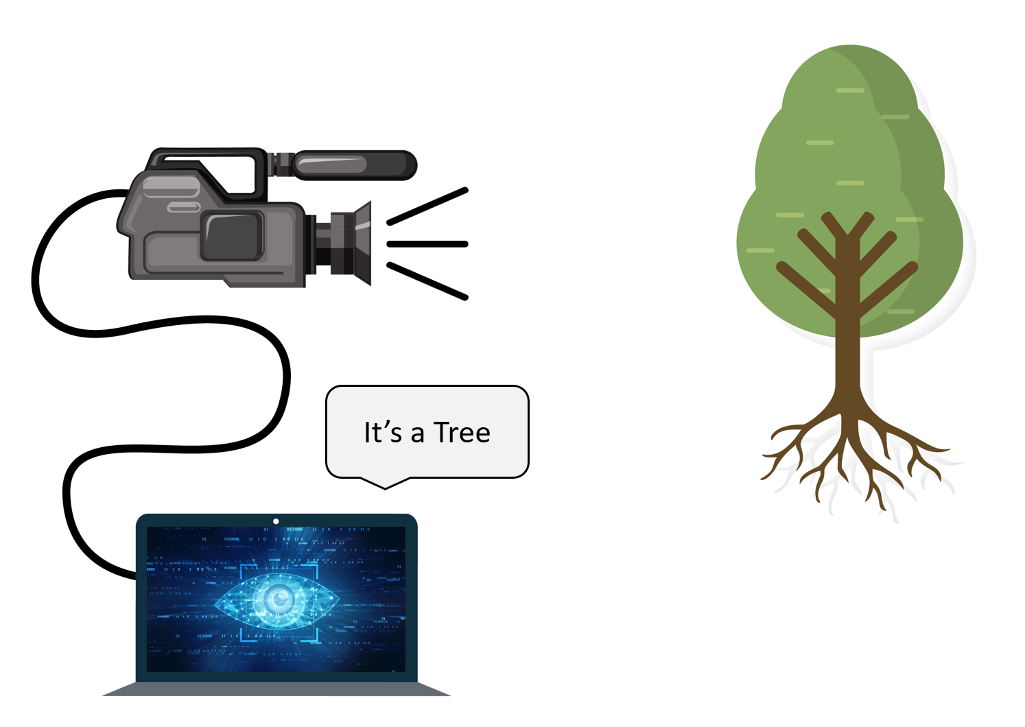
“Computer Vision is just a field of AI that enables computers or machines to see and understand the world and the things in it”
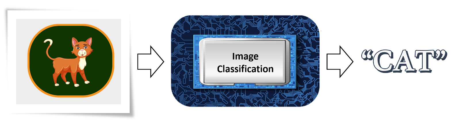
Image Classification
A very basic and popular problem in Computer Vision is Image Classification where you take an image and tell about the contents of the image.
So for e.g. A computer vision system that looks at an image of a cat and is able to recognize it.
Let’s take a look at some popular use cases of image classification systems.
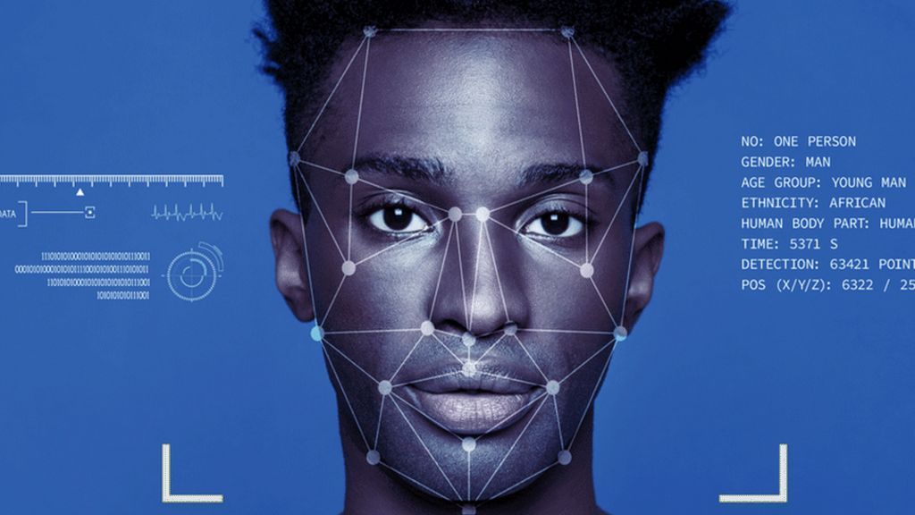
Facial Recognition:
There are many industrial use cases of classification systems and their variations. A popular application is Facial Recognition.
Where a computer program can recognize and identify the people in images by analyzing their faces. Facial Recognition is used almost everywhere from employee attendance to unlocking mobile phones.
It’s even used by Facebook to tag people, It identifies people in uploaded images/videos and automatically suggests to tag them if they’re in your mutual friends, etc.
Barcode + QR Code Scanners:
Barcode and QR Code scanners on your phones are also using this technology. It reads the machine-readable patterns and decodes them into human-readable information.
So these were some Computer Vision applications that utilizes some element of image classification.
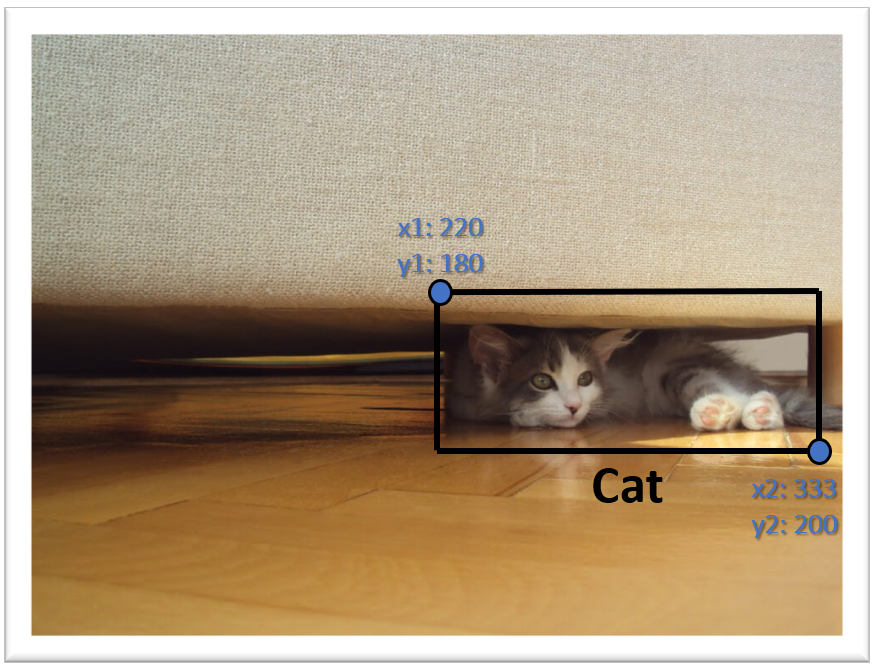
Object Detection
Sometimes we also need to extract the location of an object that is present in the image. This is when we can use Object Detection, another well-known and useful Computer Visiontask.
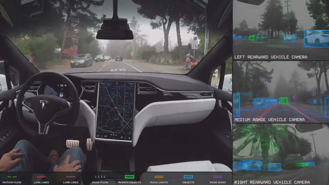
Here instead of just the label, the system also provides you with bounding box coordinates to tell where exactly the object is located in the image.
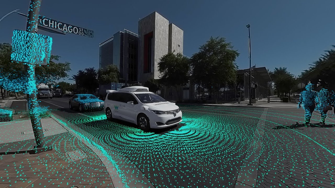
Self-driving Cars rely on Object Detection techniques to determine the location of objects like people, traffic signs, etc. This information tells the car to stop if an object is approaching it or too close to it.
Image Segmentation
Image Segmentation is another task in Vision where you try to segment or draw a pixel by pixel boundary around the object in order to segment it out. To simply put, it just partitions the pixels of the images into multiple segments (groups).
In Image Segmentation itself there are a number of techniques.
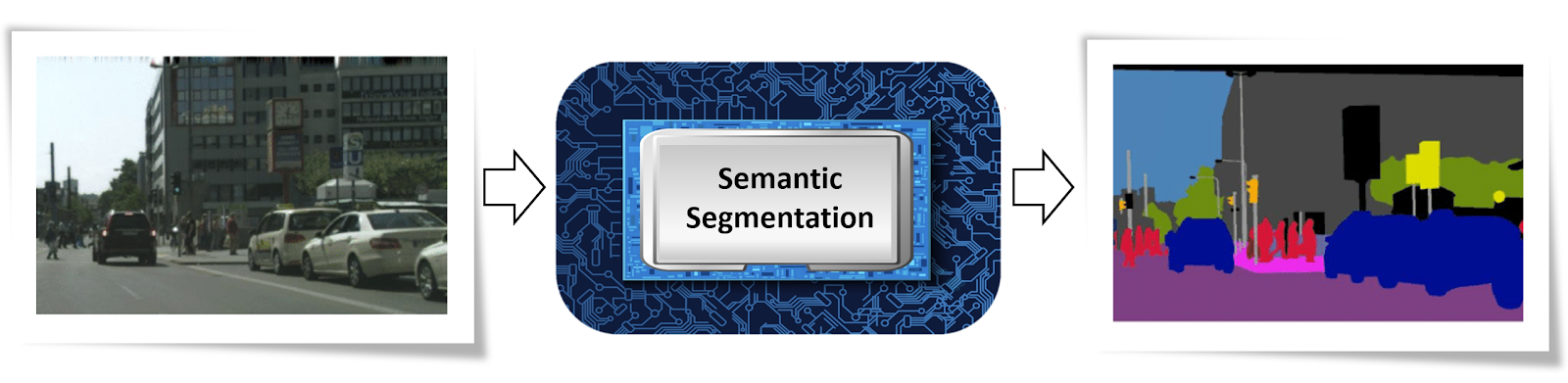
Semantic Segmentation
This approach segments the images based on the specified set of object categories/classes, which means that the objects belonging to the same category are partitioned into the same segments. For e.g. the all the cars are segmented together and you can’t separate each individual car from one another.
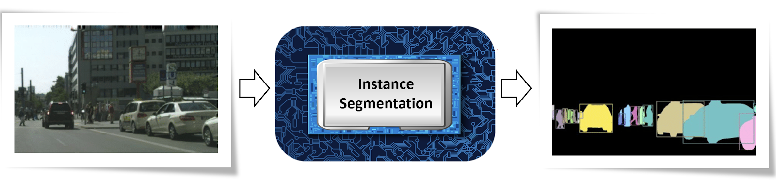
Instance Segmentation
In this method images are segmented based on the object instances, which means even if the objects belonging to the same category (e.g. cars) are partitioned into different segments. Here you can separate out each car.
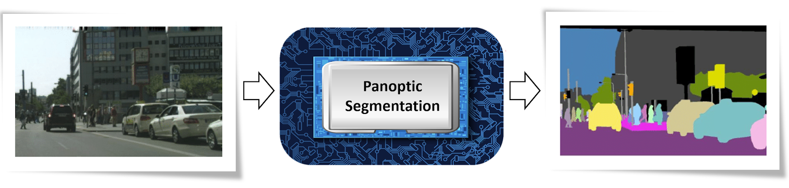
Panoptic Segmentation
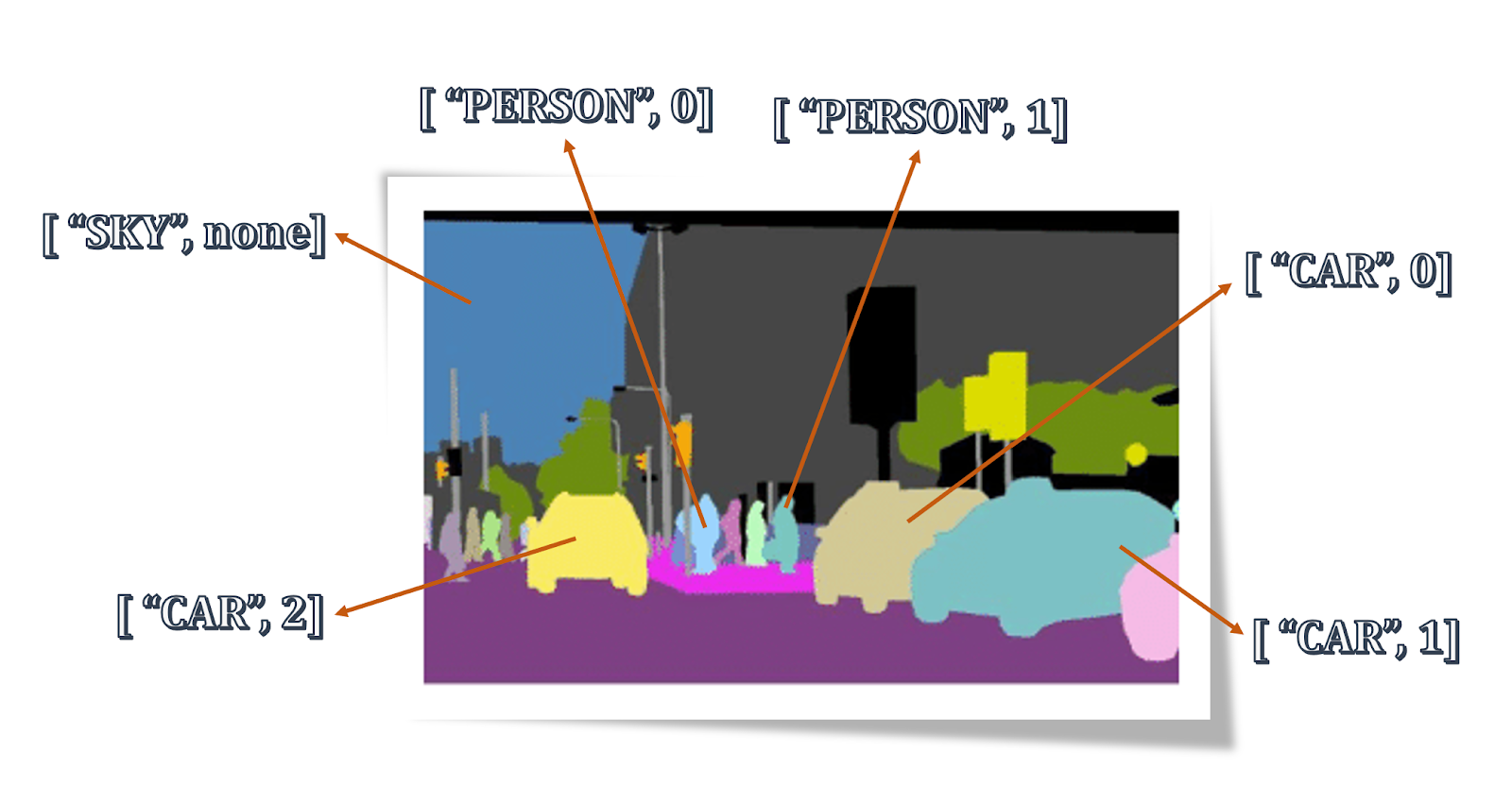
Panoptic Segmentation, on the other hand, combines both of the above techniques by segmenting the images based on both objects and instances. It assigns two labels to every pixel in the image, the first one is the semantic object category like a car, person and sky, etc and the second one is the instance id which is unique for each instance of a category.
Meeting Apps like Google Hangouts and Zoom use Image Segmentation technology to differentiate you from the background and insert custom backgrounds or blur the background behind you during the video call.
Keypoint Detection
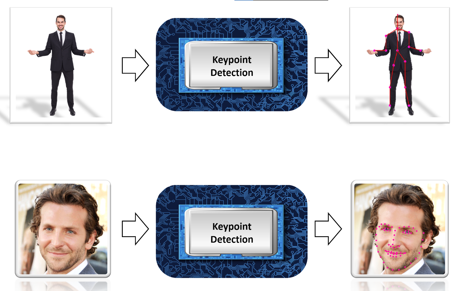
Another major vision task is called Keypoint Detection, where we try to detect some important key points on the body like a person’s body joints or his/her facial landmarks.
The key points on a person’s body joints help to determine the pose of the person whereas the key points on his/her face help in determining the facial expression of the person.
Keypoint detection is used in many human-computer interaction-based applications which allows the users to interact with the computer using their body movements.
Here are some Common industrial use cases of keypoint detection.
Keypoint Detection based applications can be used to monitor your exercise routines and provide important stats regarding your training sessions.
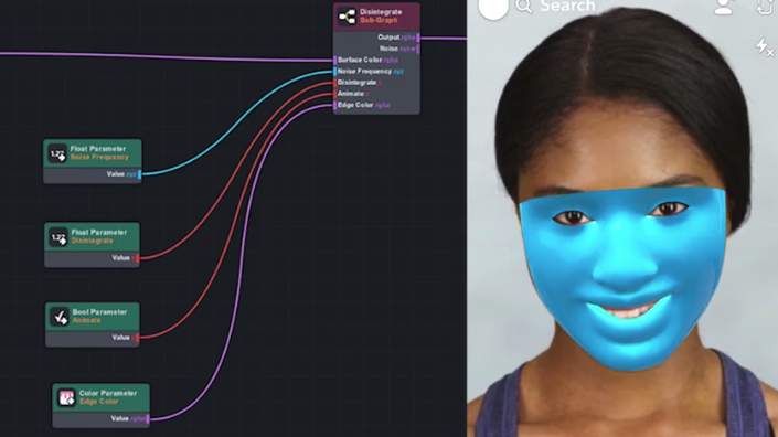
It can also be used in AR applications like Snapchat filters where different filters are triggered based on facial movement. For e.g. the Dog Filter gets triggered when a person opens his mouth, this action can be recognized by monitoring the key points around the lips.
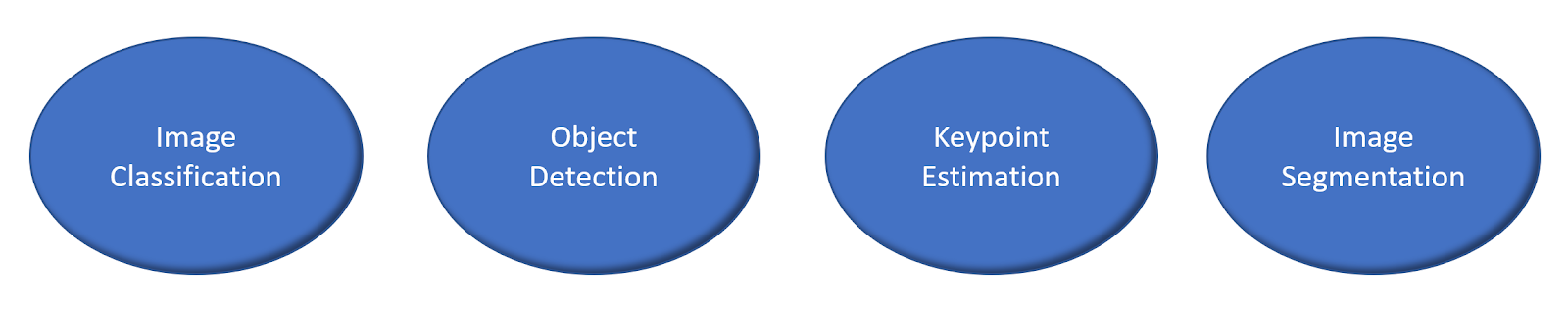
There are many other variations and types of each of these 4 core vision tasks that I have discussed.
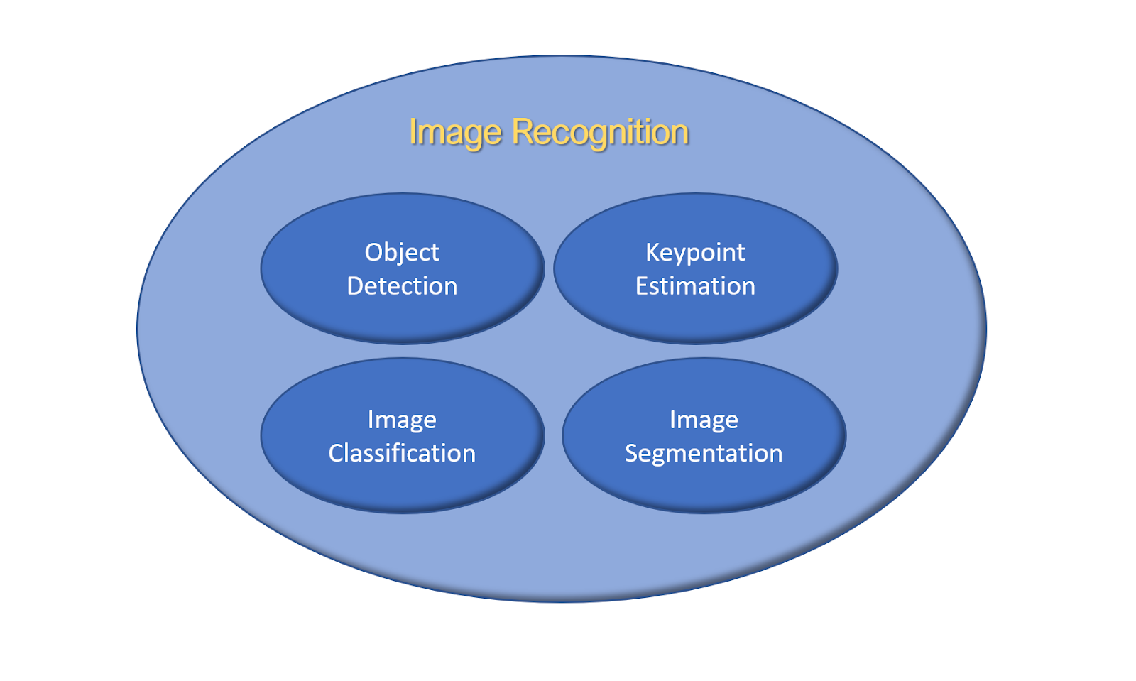
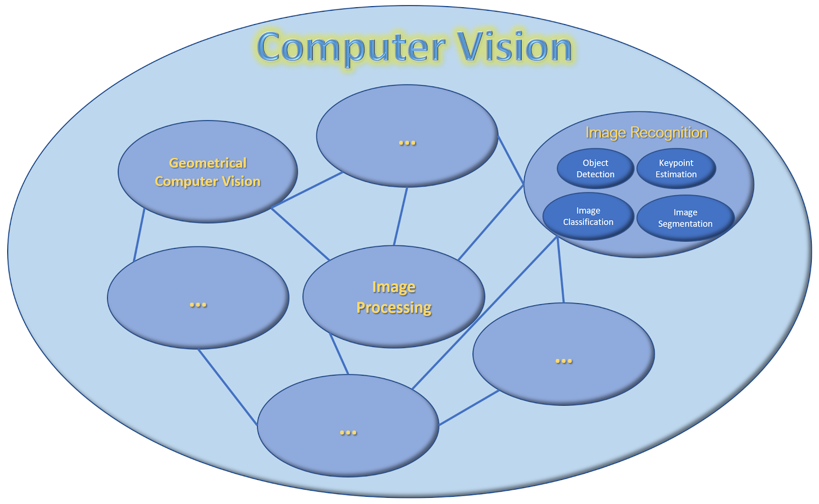
And all of these tasks loosely fall in the ”Image Recognition” sub domain of Computer Vision.
This domain deals with detecting and analyzing contents in the image. And this was just one subdomain, and there are many others like Geometrical Computer Vision, Image Processing, and others and each of them has a lot of overlap in between them.
All of these subdomains combined constitute the field of computer vision, this field gives us very interesting applications like AR filters, mixed reality, helps us automate visual tasks, provides security, and is paving the path for some really cool futuristic use cases.
There is no doubt that Computer Vision is one of the most exciting fields of Artificial Intelligence. It has a lot to offer, in the upcoming episodes, I’ll explore many of these exciting areas in computer vision so do stick around for that.
Part 2: Google Reverse Image Search
Now that you know what Computer Vision is, let me show you an amazing Computer Vision tool that you can use to level up your search skills. The tool is called “Google Reverse Image Search”
Normally when you want to search for some images you type in the search query and go to the images tab. But what if you have an image that is hard to describe (like the one below) and you want to get similar images.
That is when you should use Reverse Image Search which instead of a search query lets you search by uploading an image.
3. Then you can either paste the URL of the image or upload it from your computer and click on the Search by Image button to perform the Reverse Image Search.
When you hit the search, what google does is it uses Computer Vision to scan the image, understand its content, and then searches the internet for similar images, and finally returns the results.
After clicking the search button, you can either click on all sizes to get the exact matches of the sample image you have uploaded or click on visually similar images at the bottom to get similar images to the one you uploaded. Both of the options are highlighted in the image below.
Reverse Image Search is also really useful when you’re trying to obtain the name of a certain place, person, or a character and you only have an image of it.
For e.g. I have this image of the cat shown above and I don’t remember the name of this character, so how can I get more images like this. If I search for ninja cat, google returns me this.
Obviously not what I want. But if I use the Reverse Image Search, I get the right results as shown below.
As the tool returns all the sources which are using similar images, so content creators can also use this tool to easily search for sources on the internet that are using their images or videos.
If you’re using Chrome browser then you can also directly right-click on any image and perform Reverse Image Search by clicking on the Search Google for image option highlighted in the image below.
Fact Checking With Reverse Image Search
One really powerful and my favourite use case of reverse image search is for Fact-Checking. In this modern age of the internet, it’s quite common to see images used out of context to spread fake news.
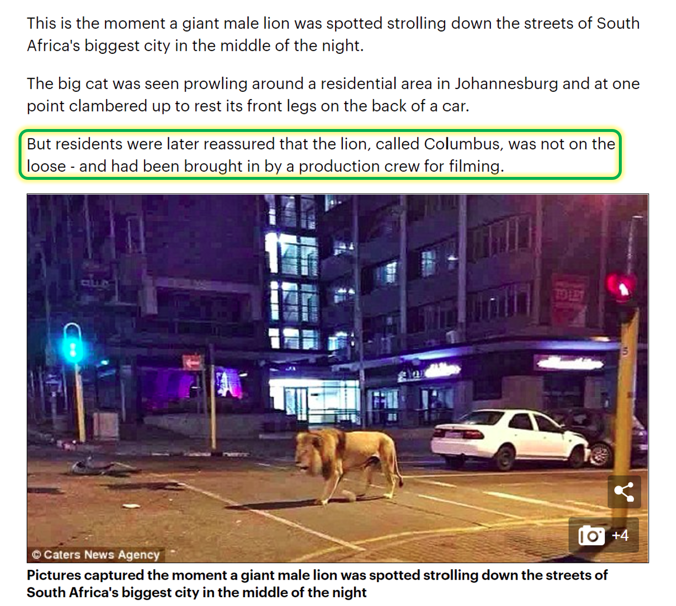
Consider this image of a lion on a street, this image went viral because some people claimed that Vladimir Putin has released lions on the streets of Russia to enforce lockdown during the pandemic. I know how absurd this sounds but believe it or not, many people actually thought this was true.
There’s another version of this image shown below where you actually get to see a fake news banner on it.
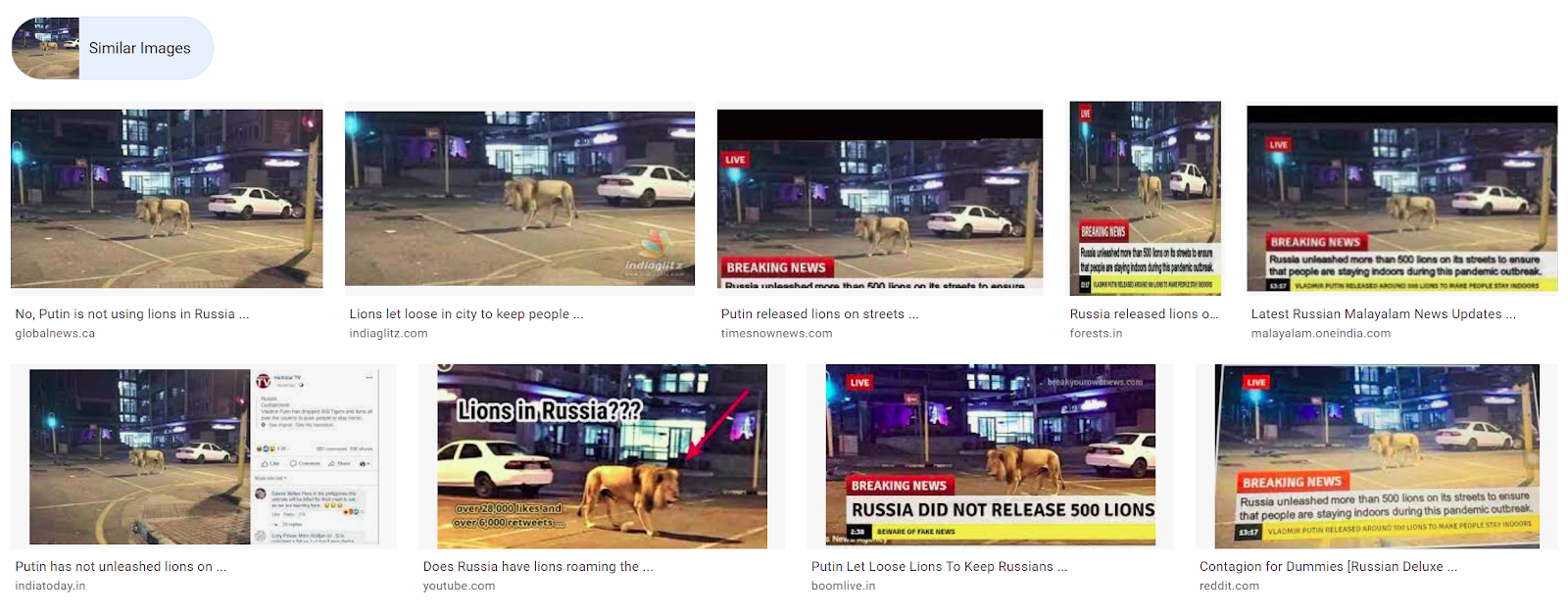
Now what people could have done is use Reverse Image Search on this image and then they would have gotten these results (see image below), where multiple news outlets debunked the lion image and revealed that it was actually an image taken during a movie production.
By clicking on any of the above returned links, you’ll see a description of the origin of the actual image.
Now that you have learned how to use this tool, you can always perform fact-checking of an image before sharing and spreading it.
Summary
In this tutorial, not only you got a high-level introduction to the field of Computer Vision but you also learned to use a very useful Computer Vision tool. In the next episode, I’ll talk about AI in general and its impact on the world. It’s going to be a very interesting post.
Note: A video-based version of this tutorial is on our youtube channel so so go check it out here.. And do make sure to subscribe to the Bleed AI channel so that you get notified when the video version comes out.
[optin-monster slug=”jmuiqewsrjgcgylo5bhj”]
You can reach out to me personally for a 1 on 1 consultation session in AI/computer vision regarding your project. Our talented team of vision engineers will help you every step of the way. Get on a call with me directlyhere.
Ready to seriously dive into State of the Art AI & Computer Vision? Then Sign up for these premium Courses by Bleed AI
Ever heard the term ‘Computer vision’ and wondered what it is? Or did you ever wanted to learn how different industries are utilizing computer vision technologies or perhaps you’re just curious about different subdomains in computer vision and want to expand your understanding in this field? Well, today we’re introducing a new video-based course that covers all that and much more called Computer Vision For Everyone.
It’s a high-level course that teaches you everything you need to get started with computer vision. The six-module course is designed in a way that people of all skill levels can benefit from it. So you don’t need any background in computer vision or Artificial Intelligence.
Not just that, this course is also useful for seasoned computer vision practitioners. And the best part is that this course is completely Free.
So if you’re still wondering, if the course is right for you then take a look at the pointers below
You want to get started in computer vision but have no idea how.
You’re excited about Artificial Intelligence but not sure where to start.
You already have some experience in Computer Vision using libraries like Tensorflow or OpenCV, but you want to get a high-level overview of all the exciting subdomains in vision.
You know how computer vision works but want to look at how different industries are utilizing this technology.
If any of the above applies to you then course if for you.
Alright, how will this course be delivered?
Well once every two weeks, you’ll get a video tutorial on an exciting topic in computer vision. The video tutorial will be released on this youtube channel, so do make sure to go there and subscribe.
Along with each video, there will also be an accompanied Blogspot which may get into more details regarding the topic and is ideal for those who prefer reading blog posts. For e.g. this post is the blogpost version of the first video episode of this course.
The course can be divided into 6 modules, In each module, we’ll cover a number of topics. Here is a list of all modules.
Module 1: Computer vision 101
Module 2: Computer Vision For Industry
Module 3: Computer Vision for Extended Reality & more
Module 4: Become a Computer Vision Ninja
Module 5: Learn to Develop Computer Vision Games
Module 6: Computer Vision As a Career
Module 1: Computer vision 101
In the first module, we’ll start with an introduction to computer vision and cover some of its applications. As we move on we’ll go over things like how an image is formed, how lenses work, compression techniques, image formats, and a lot more. We’ll understand about different subdomains in vision.
We’ll also go over the steps you need to follow to get started in computer vision and make a career in it.
And not just vision but we will also cover Artificial intelligence, machine learning, and deep learning in a very exciting way and we’ll connect and explain different AI terminologies so that things make sense.
The module sets the stage for all the upcoming modules in the series and gives you an idea of what to expect from the other lectures.
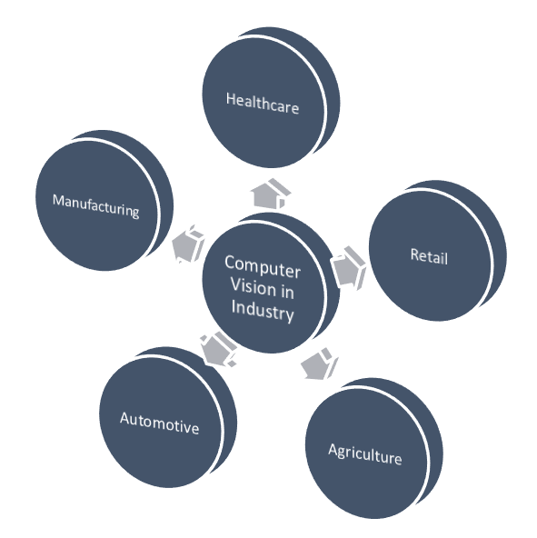
Module 2: Computer Vision For Industry
The second module explores how vision is being used for different industrial applications. We’ll understand how the Medical, Agricultural, Gaming and other industries are using Computer Vision, If you love AI applications then this module will definitely prove to be very interesting.
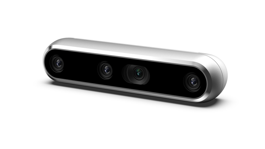
We’ll also cover things like, hardware requirements for vision, ie types of cameras used, e.g. Depth cameras, tracking cameras and everything in between and when to choose which.
Computer vision has gained popularity in recent years after major developments in deep learning but computer vision techniques are being utilized since the mid 20th century, so module two also discusses the progress made in computer vision over the years from classical techniques to deep learning-based modern approaches.
This module will also talk about the exciting research based work being done in the field, and we’ll also discuss topics like AI taking over Jobs, Threat of AI and Bias in AI and more.
Module 3: Computer Vision for Extended Reality & more
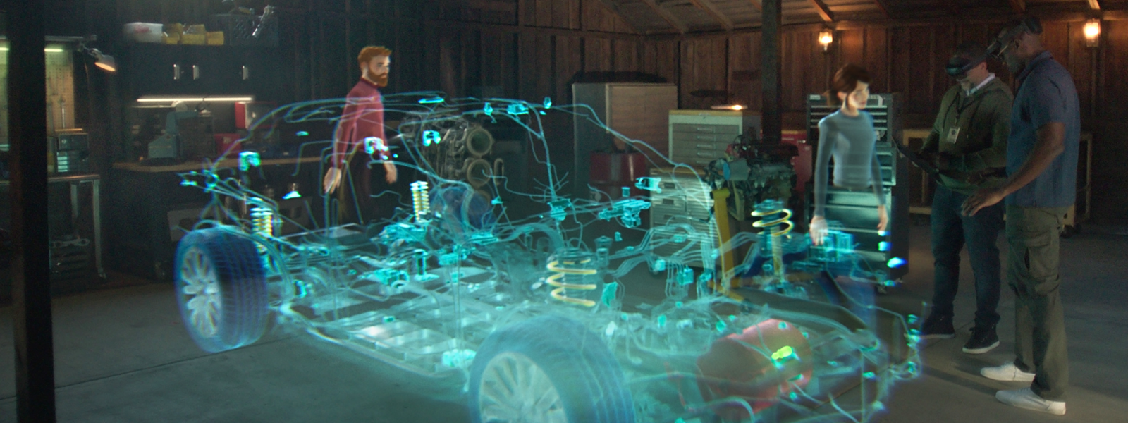
Module three is where things start to get really exciting. Vision-based augmented reality and mixed reality applications are on the rise. This is the next big step not only in the video gaming industry but also in technological devices that we use in our daily lives.
So this module will discuss all Virtual reality, augmented reality, mixed reality, and the best part is that I’ll also show you how you can use some tools to develop these extended reality apps.
This module does not end there, but we’ll also go over things like smart glasses, we’ll learn how holograms work , We’ll talk about Generative adversarial Networks and learn about Deep Fakes.
Finally we’ll wrap this module up by also discussing digital forensic techniques so you can be smart enough to recognize fake images.
Module 4: Become a Computer Vision Ninja
Building upon the momentum of the previous module, module 4 explores more into getting Hands-on experience using computer vision tools.
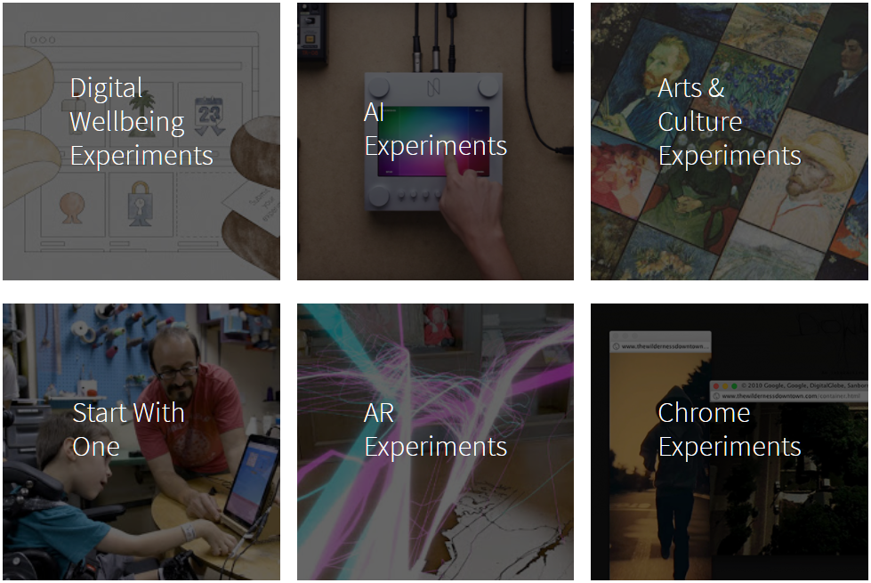
So in this module we’ll explore and learn to use Vision tools and applications in Google Experiments. Not only that, but here I’ll also discuss how each tool works and the technology behind it.
Other than google experiments, I’ll also cover some other SAS based cool vision tools that you show off to your friends.
After this module you’ll have a much better understanding regarding how to build Computer Vision based applications.
Module 5: Learn to Develop Computer Vision Games
Yes! You read that right, in this module you’ll get to develop computer vision based games. Now obviously these won’t be as cool as many production level games out there. But in this module you will learn to create simple Augmented reality based games using a popular tool called Scratch. This tool does not require any programming or any other prerequisites. Scratch will not only allow you to create games but after this module you’ll also be able to create things like animations, art, movie-like stories, program robots, and m
Module 6: Computer Vision As a Career
Computer Vision Engineer and Data Scientist is one of most in-demand job titles. After 5 modules many of you would probably want to pursue a career in computer vision so the sixth and final module will answer some important questions about making a career in computer vision. You will also learn about the best resources in vision, e.g. the best books, courses, tutorials etc.
I’ll also cover what type of projects you should work on to build up your portfolio, and finally how to get a job in computer vision.
Conclusion:
As you can tell, the course is packed with a lot of stuff. And I promise each topic will be delivered and explained with a high quality video along with an associated post, there will also be some things that I will add on to the course along the way. So do make sure to support use by subscribing to our youtube channel and sharing the videos.
[optin-monster slug=”e0ax7vpzi5iwt6zfixyy”]
You can reach out to me personally for a 1 on 1 consultation session in AI/computer vision regarding your project. Our talented team of vision engineers will help you every step of the way. Get on a call with me directlyhere.
Ready to seriously dive into State of the Art AI & Computer Vision? Then Sign up for these premium Courses by Bleed AI
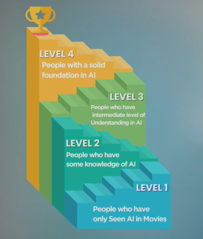
In the previous post on computer vision, we gave the simplest possible introduction to computer vision and its domains. But computer vision itself is a part of a larger domain known as Artificial Intelligence. Understanding this domain is crucial to be able to connect the dots between different fields in artificial Intelligence. So today we’re publishing a 4 part tutorial/video series on AI as part of our CVFE course, we will focus on giving you a thorough understanding of the artificial intelligence field with these 4 tutorials. Each tutorial is distributed into different levels, on each level we’ll cover some explanation of AI. And on each subsequent level, the explanations will get more technical.
So this tutorial (Level 1) will give you a high-level introduction to AI but the following posts will go deeper, exploring many of the technical aspects of Artificial Intelligence.
With that in mind, let’s just get started.
Introduction:
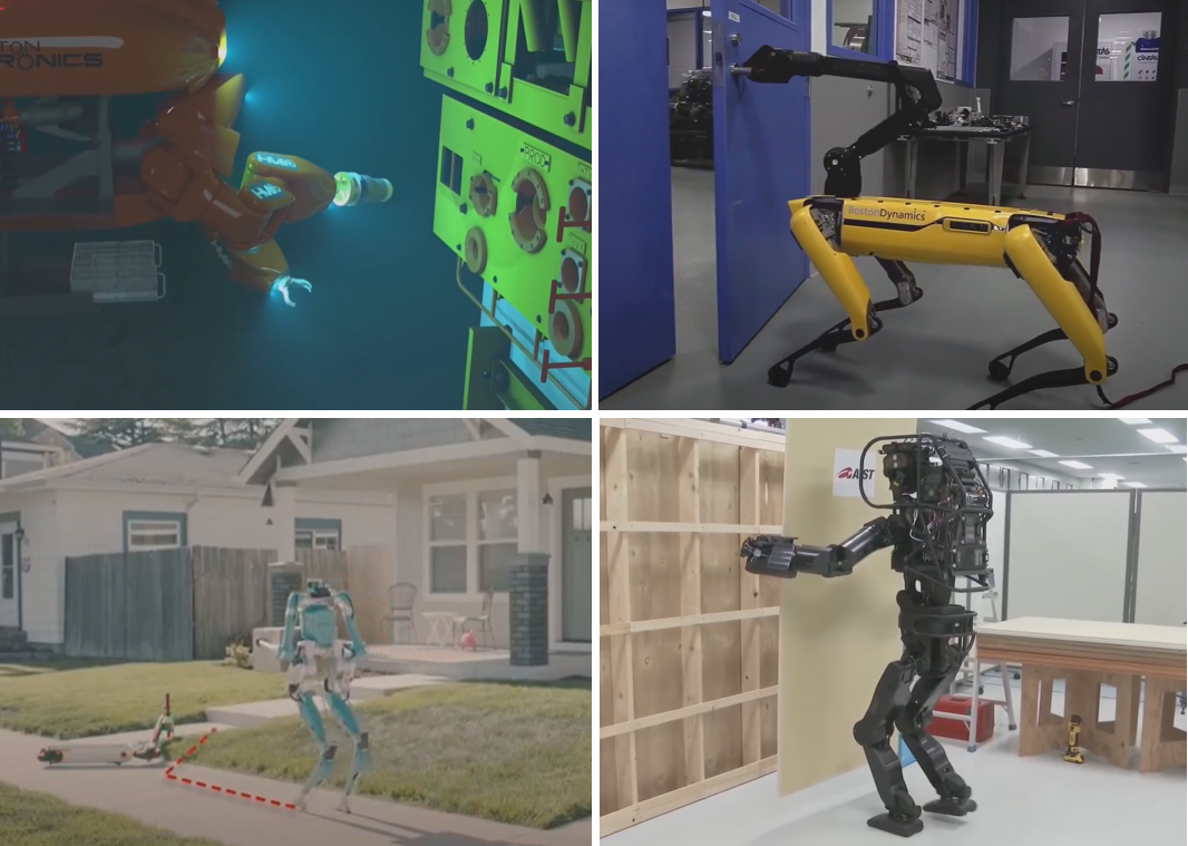
Most people develop their notion of Artificial intelligence from watching humanoid robots in media performing crazy stunts, or self-driving Teslas on the highway, or the Chinese smart surveillance systems you often hear about in the news. Perhaps you might have come across Smart stores like Amazon Go and wondered what sorcery is this?
Sci-fi books, movies, and TV series have also built our perception of Artificial Intelligence for the longest time. Movies like Terminator and Matrix introduced us to highly advanced conscious artificial intelligence systems while shows like Black-mirror painted a picture of a dystopian future where Artificial Intelligence dictates different aspects of our life.
All of this makes you wonder what the future holds for us when it comes to AI.
While many of the incredible AI systems from Sci-fi have been implemented in some shape or form, there is still a long way to go before we expect true consciousness from an Artificial system. What people need to understand is that artificial intelligence systems today can be categorized into one of the following:
ANI(Artificial Narrow Intelligence)
AGI(Artificial General Intelligence)
ASI(Artificial Super Intelligence)
For now, let’s focus on AGI and ANI, often also referred to as Strong AI and Weak AI.
AGI VS ANI:
Artificial General Intelligence, as you can tell by the name, AGI possesses intelligence comparable to humans. They can perform tasks that require the level of cognitive abilities a human mind possesses. This is the type of AI that you usually see being depicted in movies in the form of characters such as Terminator, who is able to drive vehicles, shoot weapons and use all of his senses to achieve a certain goal.
But you probably haven’t come across such a killer bot yet. This is because, in reality, the progress we have made in Artificial General Intelligence is limited. What you usually hear about in the news media are actually great examples of ANI Systems, Artificial Narrow Intelligence.
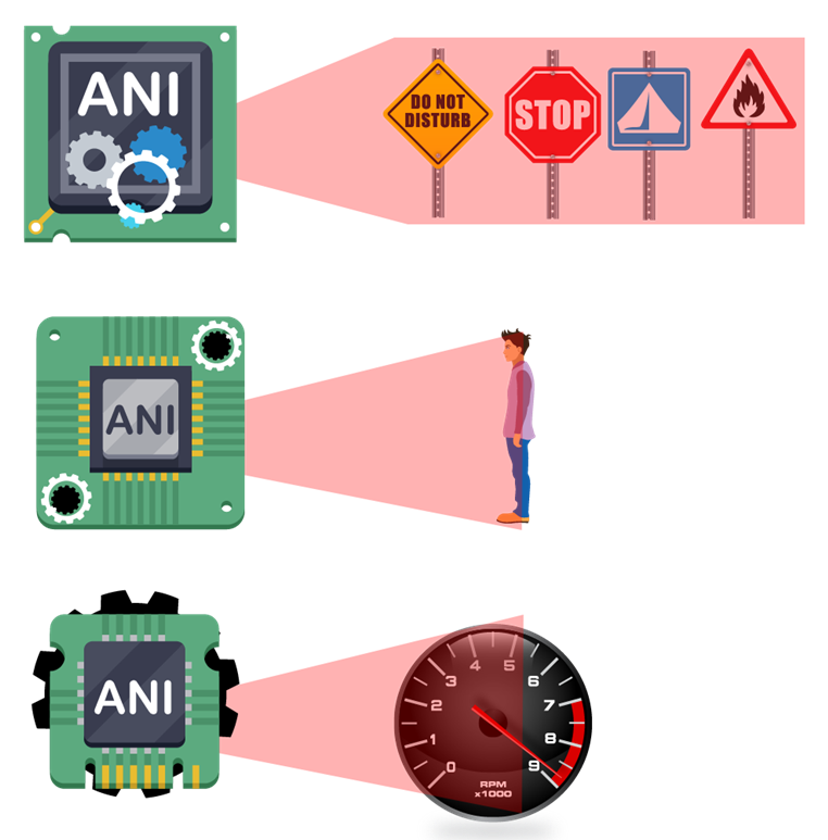
ANI (Artificial Narrow Intelligence)
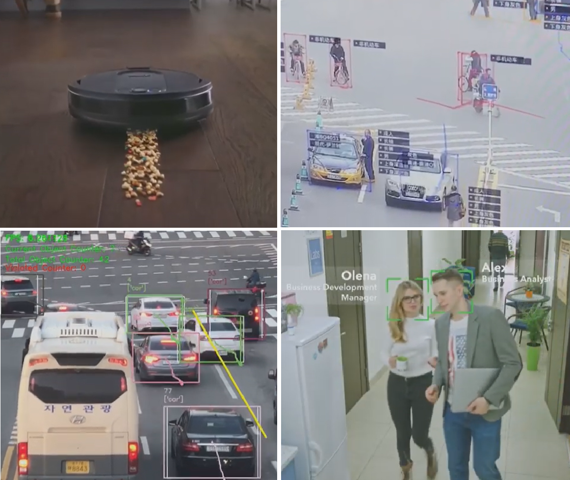
In comparison to AGI, an ANI system focuses on carrying out single specialized tasks like recognizing faces, monitoring for a restricted activity, or detecting traffic violations. Though the ANI system is limited to performing a single task, it does it really well.
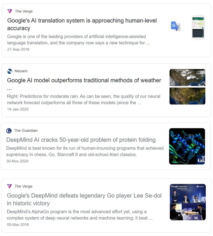
Most of the progress in artificial intelligence has been focused on building ANI systems which have also been well reflected in the media.
This rapid progress in ANI is because we have some clearly defined blueprints for developing such systems and the promising results that it yields. The healthcare industry, for example, has made significant advances in developing ANI systems capable of performing better diagnostics than human experts, which is also a lot faster and cheaper. This has the potential to impact and save thousands of lives.
As progress in ANI continues rapidly, we will witness more and more such systems deployed in different industries. Hence making an extraordinary impact.
Now you may wonder about virtual assistants like Apple’s Siri or Google’s Assistant on your smartphone, or a self-driving Tesla.
They sure seem to get a lot of stuff done at a time, so are they examples of AGI? How Can ANI take care of so many tasks at a time? Take the example of self-driving cars, not only do they steer the vehicle or control speed but they also have to watch out for pedestrians and other vehicles, or process all traffic signs signals on the road, all while maintaining an optimal course to the destination.
It sure seems a bit overwhelming for an ANI system to do all of this and you will be correct to think it’s not possible for ANI. But is it AGI then? Well not exactly, these sort of complex systems are made simply by combining smaller ANI systems that each handle a single task. Though this may give an illusion of AGI, it is simply a number of ANI systems working together.
Using multiple ANI systems together to do a complex task is hard and perhaps this is one of the reasons we still haven’t witnessed the big claims made by autonomous industry come to reality.
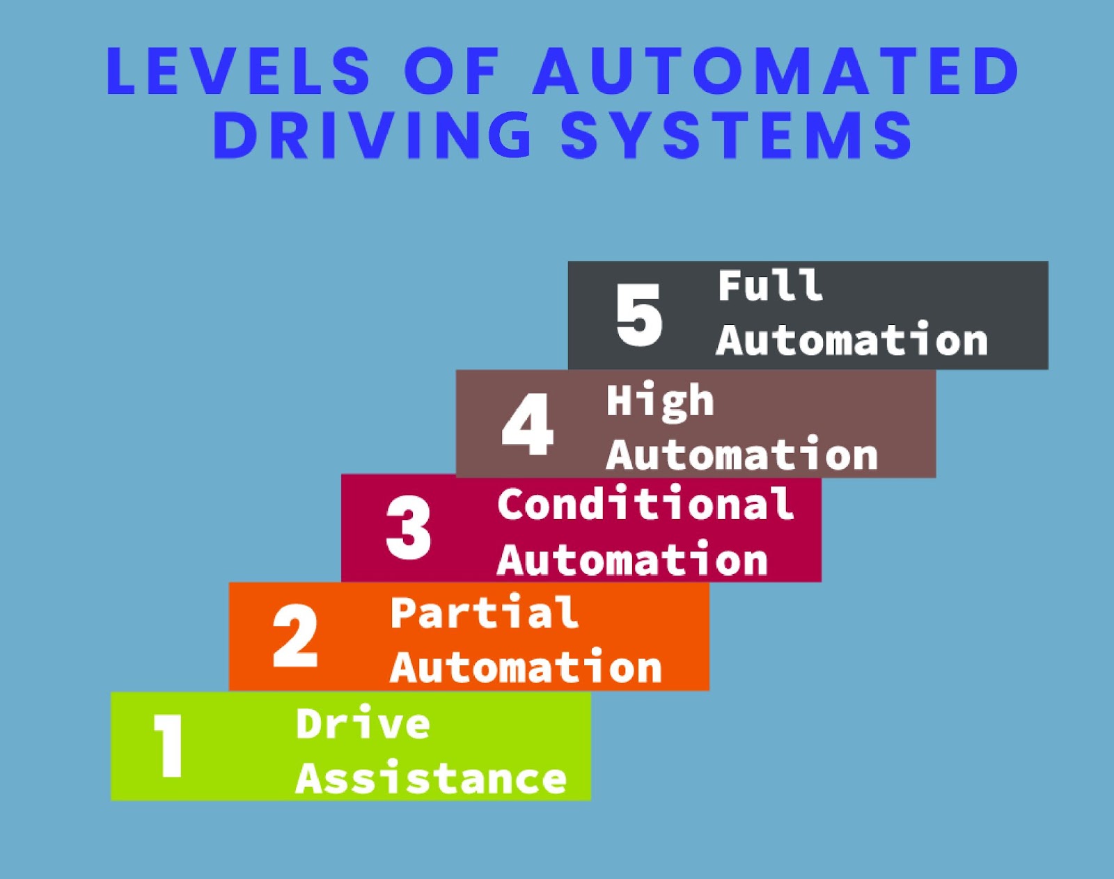
The thing that most people don’t seem to understand is, despite the advances we have made in Artificial Intelligence it’s still really hard for us to mimic human-level intelligence. Even if autonomous cars reach mass adoption, they will be in a restricted environment. I personally don’t expect to see a level 5 autonomous car before a decade. A level 5 autonomous car means a car that can autonomously drive anywhere on the planet without any human intervention. It’s a really difficult task.
Artificial Super Intelligence (ASI):
Another less discussed category in AI is called ASI, which stands for Artificial Super Intelligence. This is just like an AGI that can do all tasks a human can, but additionally, it also possesses intellectual abilities superior to humans. So theoretically an ASI system would outperform a human at any given task.
Two examples of an ASI system that you may have been familiar with are Skynet from terminator and Vision from Avengers.
ASI is also said to be capable of self-awareness meaning it can develop a consciousness.
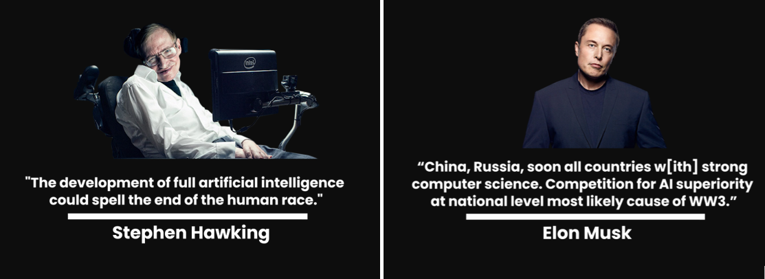
and this is the same AI that people like Elon Musk and Stephen Hawking have warned us about.
But as of now, ASI is just a hypothetical concept. So should you worry about ASI rising as a threat to humans in near future?
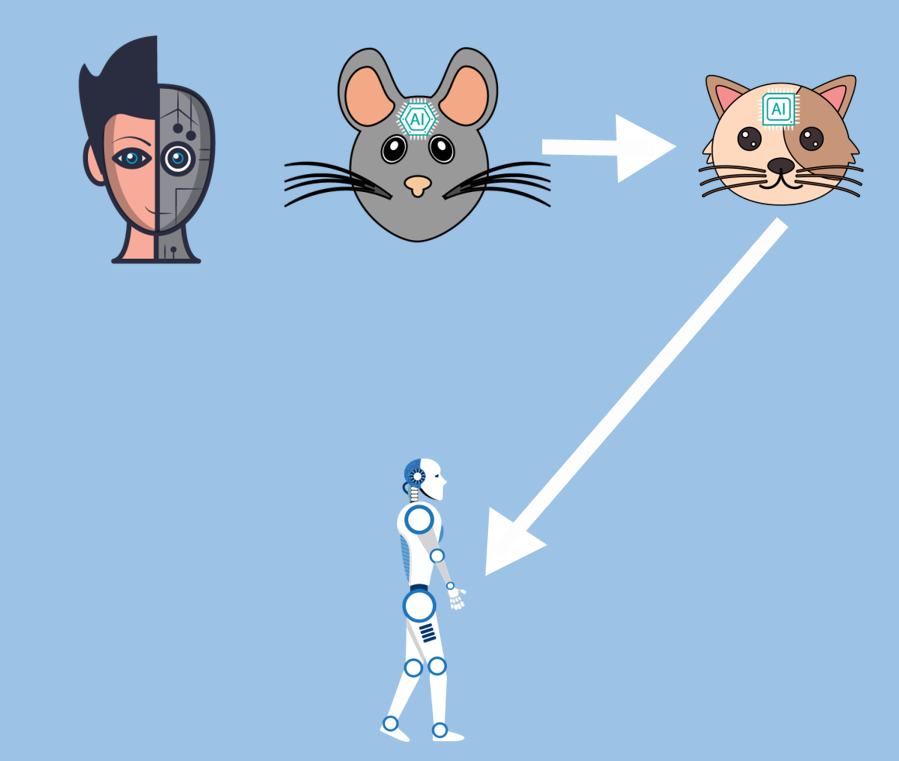
Personally, I actually don’t see humans, creating even AGI systems that can rival/surpass a human brain in our lifetime. But this is just my personal opinion. The thing is, an AGI system requires a framework or a set of algorithms that can encode and learn “common sense” and we haven’t seen much success in that department for decades. Even if we were to make progress there, it’s not like we would jump straight to human-level AGI systems. But rather first we will create systems that can demonstrate rat-level intelligence and then try to build systems for cat-level intelligence and then bit by bit go all the way to human-level intelligence.
This is a long journey requiring countless innovations and major breakthroughs in the field of AI.
SUMMARY:
ANI systems are successfully being used in multiple industries and it’s being widely adopted at an unprecedented pace. This trend will continue in the upcoming years, AI would continue to evolve and you would see AI taking up tasks and jobs that some of us are doing right now.
But there are still concerns about the democratization of AI which need to be addressed, like how it deals with bias in the real world.
Also, AI in the future will be heavily used in weaponry and to track all aspects of your life, but all those systems will be dictated and controlled by people. So AI itself is not something to be feared, the greatest threat to humanity is not AI, it is and always has been humans themselves.
With this we conclude level 1, in the next episode and Level 2 of the series, I’ll go over the history of AI and we’ll understand how we came to machine learning and deep learning. It’s going to be a very interesting post where we will dive deeper into AI.
In case you have any questions, please feel free to ask in the comment section and share the post with your colleagues if you have found it useful.
Make sure to Subscribe to Bleed AI YouTube channel to be notified when new videos are released.
[optin-monster slug=”mxcbtqsfdyknrzfguzta”]
You can reach out to me personally for a 1 on 1 consultation session in AI/computer vision regarding your project. Our talented team of vision engineers will help you every step of the way. Get on a call with me directlyhere.
Ready to seriously dive into State of the Art AI & Computer Vision? Then Sign up for these premium Courses by Bleed AI
This video is a part of our upcoming Building Vision Applications with Contours and OpenCV course. In this video, I’ve covered all the basics of contours you need to know. You will learn how to detect and visualize contours, the various image pre-processing techniques required before detecting contours, and a lot more.
The course will be released in a couple of weeks on our site and will contain quizzes, assignments, and walkthroughs of high-level Jupyter notebooks which will teach you a variety of concepts.
Download the code for the video by clicking the button below:
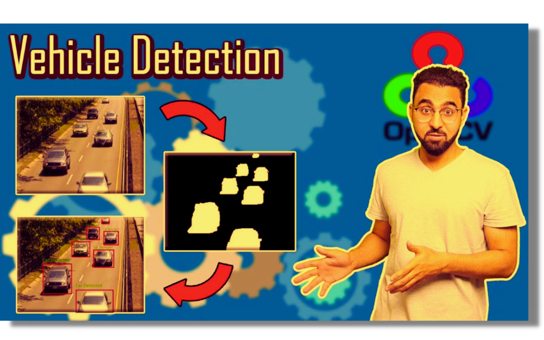
In this video we will explore how you can perform tasks like vehicle detection using a simple but yet an effective approach of background-foreground subtraction. You will be learning about using background-foreground subtraction along with contour detection in OpenCV and how you tune different parameters to achieve better results.
Download the code for the video by clicking the button below: