Teachable Machine Version 1 (Google AI Experiments)
In this video lesson I’ll teach you how to create an Image Classifier without actually coding. For this I’m using Teachable Machine version 1 which is part of Google AI Experiments. This application allows you to create image classifiers and introduces computer vision to new comers in a really fun and exciting way. I also go in the technical working of this application so people who already have some fundamental knowledge about about building classifiers can benefit from this.
Here’s the link to access this amazing tool. This is version 1, version 2 of this has also been released which deals with pose and voice recognition and even lets you export the models.
I’m offering a premium 3-month Comprehensive State of the Art course in Computer Vision & Image Processing with Python (Urdu/Hindi). This course is a must take if you’re planning to start a career in Computer vision & Artificial Intelligence, the only prerequisite to this course is some programming experience in any language.
This course goes into the foundations of Image processing and Computer Vision, you learn from the ground up what the image is and how to manipulate it at the lowest level and then you gradually built up from there in the course, you learn other foundational techniques with their theories and how to use them effectively.
Hire Us
Let our team of expert engineers and managers build your next big project using Bleeding Edge AI Tools & Technologies
You can reach out to me personally for a 1 on 1 consultation session in AI/computer vision regarding your project. Our talented team of vision engineers will help you every step of the way. Get on a call with me directlyhere.
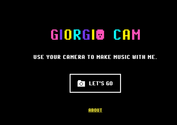
This Video goes covers Giorgio Cam which is a part of Google AI experiments. In this video I explain how you can convert images or object images to actual song lyrics using Giorgio Cam. So basically this is doing Image recognition to recognize the contents in the image and then uses Speech synthesis to convert the results of recognition to some lyrical sentence.
A lot more is happening in the background and I also went into the technical working of this application so you can build something on top of it or at least be inspired enough to build something cool.
I’m offering a premium 3-month Comprehensive State of the Art course in Computer Vision & Image Processing with Python (Urdu/Hindi). This course is a must take if you’re planning to start a career in Computer vision & Artificial Intelligence, the only prerequisite to this course is some programming experience in any language.
This course goes into the foundations of Image processing and Computer Vision, you learn from the ground up what the image is and how to manipulate it at the lowest level and then you gradually built up from there in the course, you learn other foundational techniques with their theories and how to use them effectively.
Hire Us
Let our team of expert engineers and managers build your next big project using Bleeding Edge AI Tools & Technologies
You can reach out to me personally for a 1 on 1 consultation session in AI/computer vision regarding your project. Our talented team of vision engineers will help you every step of the way. Get on a call with me directlyhere.
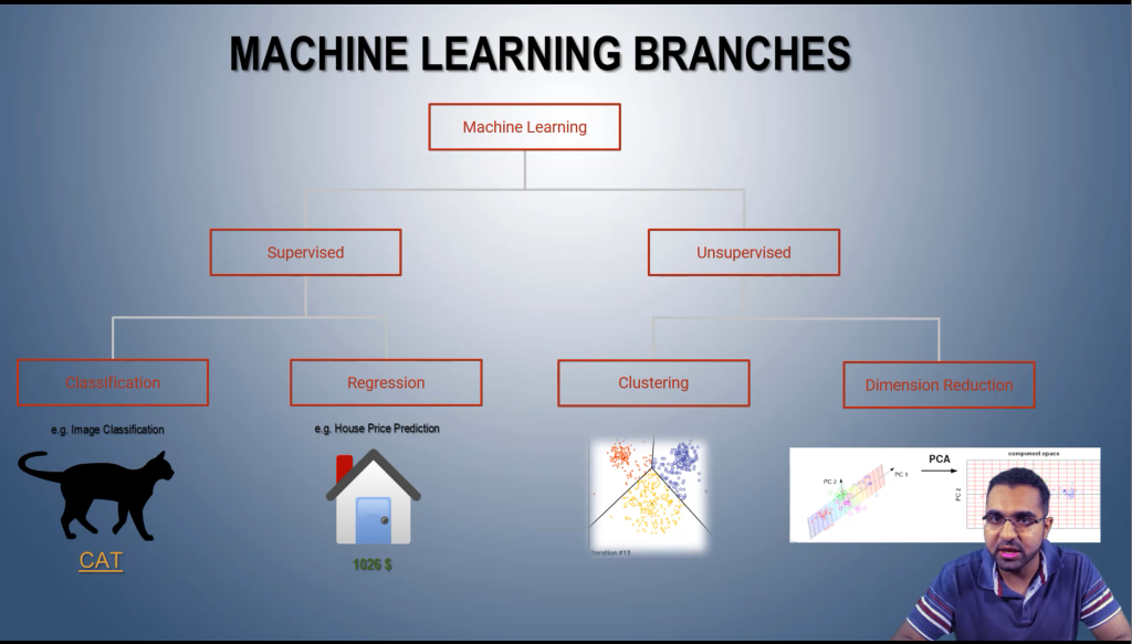
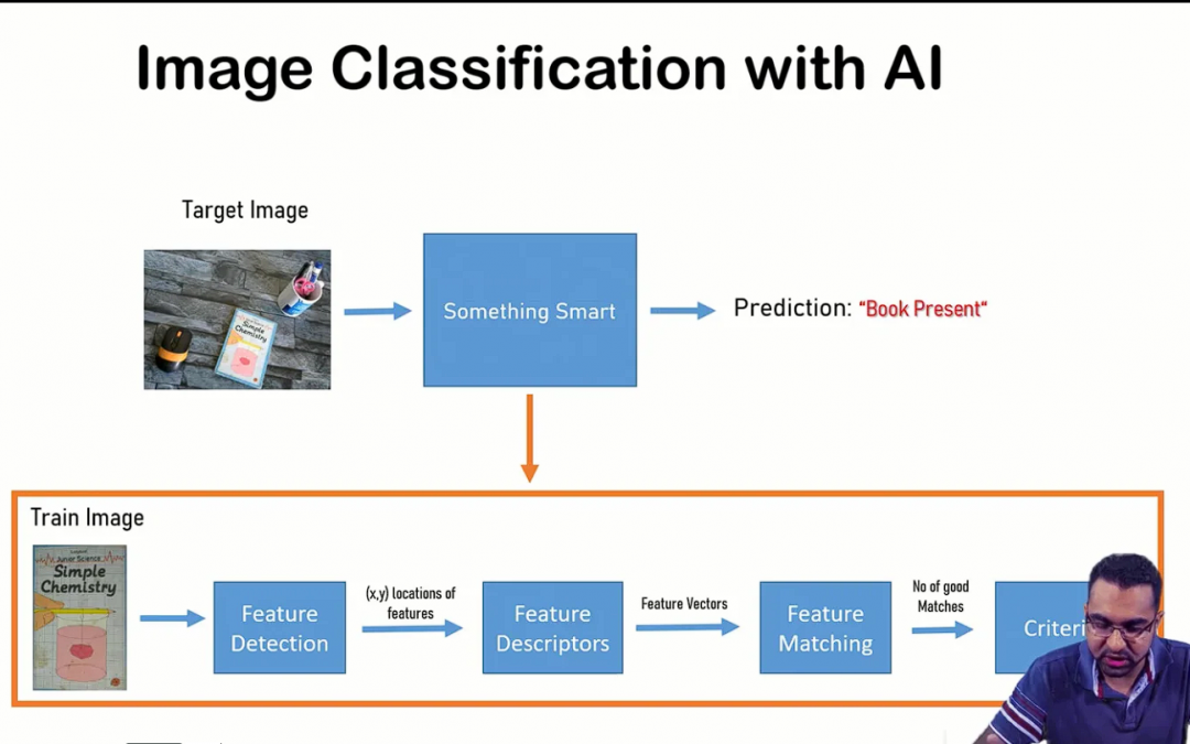
In this Video I go Over 10 Different Ways To Perform Image Classification. I also Cover how you Would perform Classification with Traditional AI, with ML & finally with DL.
I’m offering a premium 3-month Comprehensive State of the Art course in Computer Vision & Image Processing with Python (Urdu/Hindi). This course is a must take if you’re planning to start a career in Computer vision & Artificial Intelligence, the only prerequisite to this course is some programming experience in any language.
This course goes into the foundations of Image processing and Computer Vision, you learn from the ground up what the image is and how to manipulate it at the lowest level and then you gradually built up from there in the course, you learn other foundational techniques with their theories and how to use them effectively.
Hire Us
Let our team of expert engineers and managers build your next big project using Bleeding Edge AI Tools & Technologies
You can reach out to me personally for a 1 on 1 consultation session in AI/computer vision regarding your project. Our talented team of vision engineers will help you every step of the way. Get on a call with me directlyhere.
Have You seen those Sci fi movies in which the detective tells the techie to zoom in on an image of the suspect and run an enhancement program and suddently that part of image is magically enhanced to a higher resolution instead of being pixelated.
Feel free to take a look at a compilation of those exact scenes below.
It’s also absurd, the amount of times that they all got a reflection of something in the video. Anyways the point is that in the past few years we have made that aspect of Sci-fi a reality. Meaning today with deep learning methods we can actually enhance many low-resolution images to a high-resolution version, sometimes even as high as 8x resolution. This means you can take a 224×224 image and make it 1792×1792 without any loss in quality. This technique is called Super Resolution.
In this tutorial you will learn how to perform Super-Resolution with just OpenCV, specifically, we’ll be using OpenCV’s DNN module so you won’t be using any external frameworks like Pytorch or Tensorflow.
Before we start with the code I want to briefly discuss the amazing progress of Super-Resolution Algorithms. You can feel free to jump right into the code. But I would recommend giving the theory below a quick read even if you don’t understand all of it.
So technically speaking, Super Resolution can be defined as the class of Algorithms that upscales an image without losing quality. How would you upscale an image without this? well you could say you can resize the image and make it larger.
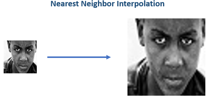
So when you typically resize an image, you use Nearest Neighbor Interpolation. This just means you expand the pixels of the original image and then fill the gaps by copying the values of the nearest neighboring pixels.
Figure 1: Nearest Neighbor interpolation.
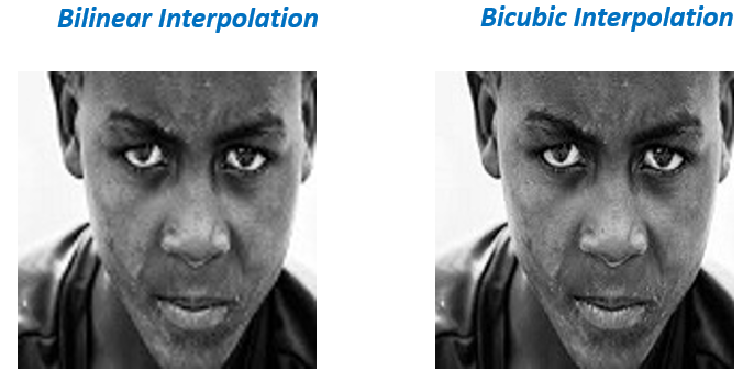
Of Course the results would be terrible, you can do better by taking a weighted average of neighboring pixels instead of just copying them. This is essentially done by using Bilinear or Bicubic interpolation.
Still the results above are blurred and you can easily tell that its not the original version. So can we make this upscaled version look like the original with some fancy Algorithms? Well the short answer is `No`. No smart function or algorithm will be able to replace the missing information. The best we can do is approximate and fill the gaps based on the neighboring pixels.
But fret not, Neural Networks come to the rescue. These algorithms can actually look at thousands of samples and remember the patterns so at the end of the day you don’t have to approximate the missing information, you can hallucinate based on the past seen data.
They simply input Low res (downscaled version) of images and made the model output a Higher resolution version and then compared it with the original High res version. The metric they were Optimizing was Peak signal to noise ratio (PSNR) score.
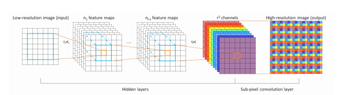
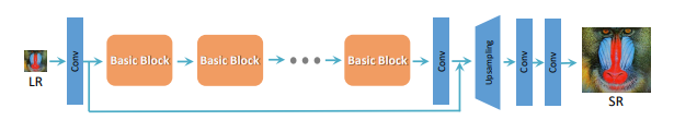
SRResNet (Real-Time Single Image and Video Super-Resolution Using an Efficient Sub-Pixel Convolutional Neural Network ) in 2016 by Wenzhe Shi et al improved upon the previous SRCNN at two levels, first, it used Residual blocks (Convolution layers with skip connections) instead of normal Convolution layers. Why? Well the success of architectures like ResNets made the fact popular that Residual blocks are more powerful than simple convolutional layers, as it allowed to add more layers without overfitting.
Second, it shifted the upsampling step to the middle of the network. Now in any Super res architecture there has to be an upsampling step. Now if you’re using bicubic interpolation inside the network to upsample then you can either use it at the start or the end, you can’t use it in the middle because It’s a fix mathematical operation, it’s not learnable. Now if you want to have upsampling in between the layers then you can go for transpose layers to upsample the image. One problem tho, transpose convolutions adds zeros to upscale the image, you don’t have any gradient information to tune this upscaling process. The way SRResNet got around that was that it used sub pixel convolutions to upscale, without me explaining what this layer is you just have to understand that with this technique of upscaling is a learnable operation, so this improved results. This model was also optimizing the PSNR score.
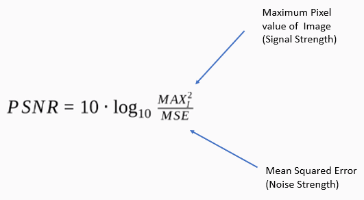
Now Consider the PSNR score again:
Figure 4: PSNR Equation
As you can see, the model will have a high PSNR score if the MSE (mean squared error) is low. Now this approach works well, but the problem here is that even with high PSNR scores the images do not necessarily look good to the human eye.
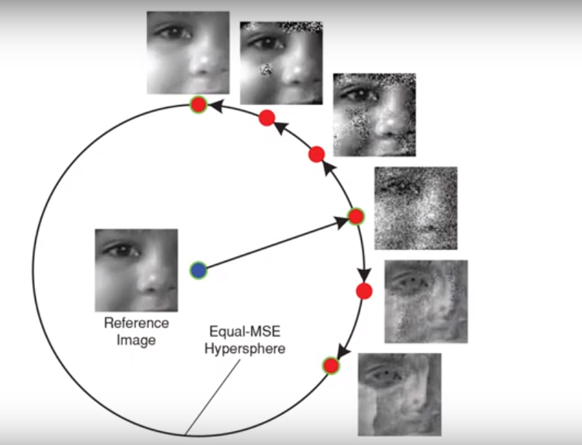
So the image fidelity or the human perception of image quality is not exactly correlated to psnr scores. Minimizing MSE would produce images that may look more like the original but may not necessarily look pleasing to the eye.
Consider all these images below that have almost equal MSE when compared to the reference image, even though we can clearly see that the image on the top is way closer to reference image than the bottom one.
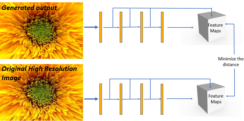
MSE only cared about pixel-wise intensity differences not the actual contents of the image. This problem can be solved by using a better metric. Something called a Perceptual loss (Perceptual Losses for Real-Time Style Transfer and Super-Resolution in 2016 by Justin Johnson et al) can be used. It’s kind of a loss that correlates well with our perception of image quality. It works by simply passing the output of the model and the actual target image to a pre-trained model like VGG variants and then compute the difference between the resulting feature maps of that model and try to minimize that. The layers of the pre-trained model that generates those feature maps for loss calculation stays frozen during the training of the Super res network. This perceptual loss is also called the content loss in style transfer networks.
For a moment if we think about the Super Resolution problem then we can agree that we don’t care if the output image matches the original one exactly as long as it looks good, So why not use GANs (Generative Adversarial Networks) to generate realistic Upscaled versions of the image. That’s what SRGAN (Photo-Realistic Single Image Super-Resolution Using a Generative Adversarial Network) Christian Ledig et al, 2017 did. Like all GANs SRGAN, had a generator that tries to generate realistic-looking Upscaled versions of the original images and it also had a discriminator that tried to tell if the generated image is the Original high res version or a generated Upscaled version. During the training they both get better over time and the generator learns to produce better looking Upscaled versions of the image.
In Addition to this, SRGAN also implemented a Perceptual loss function. So this network with the combination of Generative Loss & Perceptual Loss along with sub-pixel convolutions produces really High-quality Upscaled images.
An interesting variant of SRGANs is this ESRGAN: Enhanced Super-Resolution Generative Adversarial Networks by Xintao Wang et al, 2018. The paper did lots of simple yet interesting things like removing the Batch norm layer, doing residual scaling, modifying discriminator loss, taking feature maps comparison before the activation function, etc. to the above network and so the performance improved.
The network also computed a weighted average of two models, a GAN model and an MSE trained model, this way the Output looked real and also closely resembled the original image.
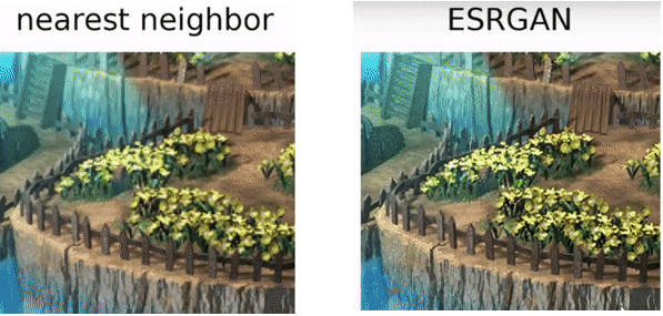
This network got pretty popular in the gaming community, people upscaled old gaming graphics.
Figure 10: Nearest Neighbor and ESRGAN in Gaming.
Other Areas Of Super Resolution:
Domain/Task Specific Super Resolution:
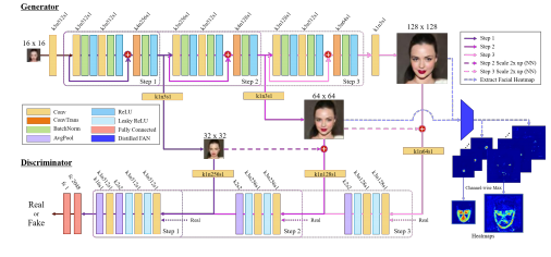
Needless to say if you train Super Res on a certain type of data then it will perform really well on that type. So people have trained really powerful Super res networks on domain problems like training only on faces and by utilizing face priors, you get a network (like this: Pixel Recursive Super Resolution) which can generate plausible high res face images from a very low res image. Of Course these types of networks can’t be used for CSI use cases as the details are totally made up by the algorithm.
All the methods discussed above belong to the “Single Image Super-Resolution” category, while most of the interesting papers in SR are in this category but there is another area called “Multi-Image Super-Resolution” in which you have multiple images of the same scenes but the camera is slightly shifted, by some subpixels on each image. Then you use that extra information from all those individual images and construct a high res version. In fact Google’s New Pixel 3 uses a Multi-Image SR algorithm that uses those slight shifts of handheld motion to produce those amazing SR Zoom effects.
Note: Super resolution is a really popular subject and you’ll see a good number of research papers published each year in this area. There are other interesting papers that I have not discussed but the papers I have mentioned in essence capture the evolution of Super res networks.
Super Resolution with OpenCV Code
Now let’s start with the code, we are going to be using OpenCV’s DNN module, this was introduced in OpenCV version 3 and now in version 4.2 it has evolved a lot. This module lets you use pre trained neural networks from popular frameworks like tensorflow, pytorch, onnx etc and use those models directly in OpenCV.
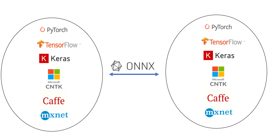
The model is in ONNX format (Open neural network exchange format). This is an industry-standard format for changing model frameworks, this means you can train a model in PyTorch or other common frameworks and then convert to onnx and then convert back to TensorFlow or any other framework.
OpenCV DNN module allows you to use models that are in ONNX format by using cv2.dnn.readNetFromONNX(). You can get a list of ONNX models from the ONNX Model Zoo.
Figure 14: ONNX model Conversion.
Here are the steps we would need to perform:
Initialize the Dnn module.
Read & Pre-process the image.
Set the preprocessed image as input and do a forward pass with the model.
Post-process the results to get the final image
Make sure you have the following Libraries Installed.
OpenCV ( possibly Version 4.0 or above)
Numpy
Matplotlib
Download Code
[optin-monster slug=”rvfkmnfpxleeisjulg1h”]
Directory Hierarchy
Make sure to download the zip folder containing the source code, images, & model from above. After downloading, extract the folder and run the Jupyter notebook kernel from there.
This is how our directory structure looks like, it has a Jupyter notebook, a media folder with images and the model folder.
Super Resolution
     │   Super Resolution.ipynb
     │
     ├───Media
     │       oldman.jpg
     │       teenager.jpg
     │       uncle.jpg
     │       youngman.jpg
     │       youngman2.jpg
     │
     └───Model
             super_resolution.onnx
Import Libraries
Start by Importing the required libraries.
# Import Required libraries
import cv2
import numpy as np
import matplotlib.pyplot as plt
import os
%matplotlib inline
Initialize DNN Module
To use Models in ONNX format, you just have to use cv2.dnn.readNetFromONNX(model) and pass the model inside this function.
model = 'Model/super_resolution.onnx'
net = cv2.dnn.readNetFromONNX(model)
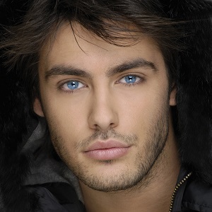
Read Image
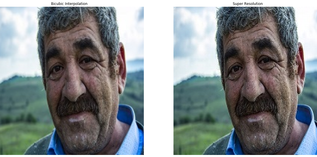
This is our image on which we are going to perform super-resolution.
Line 5-7 : We’re setting the figure size and showing the image with matplotlib, `[:,:,::-1]` means to reverse image channels so we can show OpenCV BGR images properly in matplotlib. OpenCV BGR images.
Preprocessing the image
Before you pass in an image to a neural network you perform some image processing to get the image in the right format. So the first thing we will do is resize the image to have the size 224×224. This is the size that our network requires. After that we’ll convert the image from RGB to YCbCr color format. So take a look at the components in this format.
Y: This is called the lumma component. So basically this channel encodes brightness intensity of the image, you can think of this channel like the grayscale version of the image.
Cb: This is the blue-difference channel.
Cr: This is the red difference channel.
So why are we doing this? If we try to Upscale an RGB (or BGR in case of OpenCV) Color image then we would need to train a network that would have to learn to Upscale each individual channel, so instead of doing that we can do something smarter, That changes the image to the color format where you can just manipulate the main intensity channel. So the network we’re using has learned to upscale `Y` channel. After it does that, all we do is upscale the channels (These are responsible for color) using bicubic interpolation and merge it with the Y channel. This cuts our work to 1/3. After this we do some formatting of the `Y` channel and then finally normalize it by dividing with 255.0.
# Create a Copy of Image for preprocessing.
img_copy = image.copy()

# Resize the image into Required Size
img_copy = cv2.resize(img_copy, (224,224), cv2.INTER_CUBIC)

# Convert image into YcbCr
image_YCbCr = cv2.cvtColor(img_copy, cv2.COLOR_BGR2YCrCb)

# Split Y,Cb, and Cr channel
image_Y, image_Cb, image_Cr = cv2.split(image_YCbCr)

# Covert Y channel into a numpy arrary
img_ndarray = np.asarray(image_Y)

# Reshape the image to (1,1,224,224)
reshaped_image = img_ndarray.reshape(1,1,224,224)

# Convert to float32 and as a normalization step divide the image by 255.0
blob = reshaped_image.astype(np.float32) / 255.0
Line 2-5: We’re making a copy of the image and resizing it to the size the network requires.
Line 8-11: Changing the color channel to YCbCr & splitting it to individual channels, so we can just work with the `Y` channel.
Line 14-17: Formatting Y to the format that is acceptable by the network.
Line 20: Converting to float and normalizing the image as it was done in the original implementation.
Input the Blob Image to the Network
# Set the processed blob as input to the neural network.
net.setInput(blob)
Forward Pass
Most of the Computations will take place in this step, in my PC it took 90 ms for a single pass. This is the step where the image goes through the whole neural network.
# Perform a forward pass of the image.
Output = net.forward()
Post-processing
After the network outputs the results, you need to post-process it. Mostly you reverse what you did in the preprocessing step.
# Reshape the output and get rid of those extra dimensions
reshaped_output = Output.reshape(672,672)

# Get the image back to the range 0-255 from 0-1
reshaped_output = reshaped_output * 255

# Clip the values so the output is it between 0-255
Final_Output = np.clip(reshaped_output, 0, 255)

# Resize the Cb & Cr channel according to the output dimension
resized_Cb = cv2.resize(image_Cb,(672,672),cv2.INTER_CUBIC)
resized_Cr = cv2.resize(image_Cr,(672,672),cv2.INTER_CUBIC)

# Merge all 3 channels together
Final_Img = cv2.merge((Final_Output.astype('uint8'), resized_Cb, resized_Cr))

# Covert back to BGR channel
Final_Img = cv2.cvtColor(Final_Img,cv2.COLOR_YCR_CB2BGR)
Line 2-5: We’re reversing what we did in the preprocessing step.
Line 8: Clipping to stay in the uint8 range and avoid artifacts in the final image from rounding.
Line 11-12: Resizing the color channels according to the ‘Y’ channel.
Line 15-18: Merging all channels and converting the image back to BGR.
Display Final Result
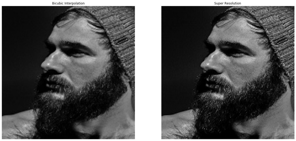
# Also Get the Bicubic interpolated version of the original image
image_bicubic = cv2.resize(image, (672,672), cv2.INTER_CUBIC)

# Display the Bicubic Image and Super Resolution Image
plt.figure(figsize=[20,20])
plt.subplot(1,2,1);plt.imshow(image_bicubic[:,:,::-1]);plt.title("Bicubic Interpolation");plt.axis("off");
plt.subplot(1,2,2);plt.imshow(Final_Img[:,:,::-1]);plt.title("Super Resolution");plt.axis("off");
Line 5-7: We’re displaying both the bicubic and super-resolution version of the image in subplots.
Creating Functions
Now that we have seen step by step implementation of the network, we’ll create the following 2 python functions.
Initialization Function: This function will contain parts of the network that will be set once, like loading the model. Main Function: This function will contain all the rest of the code from preprocessing to postprocessing, it will also have the option to either return the enhanced image or display it with matplotlib.
Initialization Function
def init_superres(model="Model/super_resolution.onnx"):
    global net
    # Initialize the DNN module
    net = cv2.dnn.readNetFromONNX(model)
Main Function
Set `returndata = True` when you just want the enhanced image. I usually do this when working with videos.
def super_res(image, returndata=False):

    # Create a Copy of Image
    img_copy = image.copy()

    # Resize the image into Required Size
    img_copy = cv2.resize(img_copy, (224,224), cv2.INTER_CUBIC)

    # Convert image into YcbCr
    image_YCbCr = cv2.cvtColor(img_copy, cv2.COLOR_BGR2YCrCb)

    # Split Y,Cb, and Cr channel
    image_Y, image_Cb, image_Cr = cv2.split(image_YCbCr)

    # Covert Y channel into a numpy arrary
    img_ndarray = np.asarray(image_Y)

    # Reshape the image to (1,1,224,224)
    reshaped_image = img_ndarray.reshape(1,1,224,224)

    # Convert to float32 and as a normalization step divide the image by 255.0
    blob = reshaped_image.astype(np.float32) / 255.0

    # Passing the blob as input through the network
    net.setInput(blob)

    # Forward Pass
    Output = net.forward()

    # Reshape the output and get rid of those extra dimensions
    reshaped_output = Output.reshape(672,672)

    # Get the image back to the range 0-255 from 0-1
    reshaped_output = reshaped_output * 255

    # Clip the values so the output is it between 0-255
    Final_Output = np.clip(reshaped_output, 0, 255)

    # Resize the Cb & Cr channel according to the output dimension
    resized_Cb = cv2.resize(image_Cb,(672,672),cv2.INTER_CUBIC)
    resized_Cr = cv2.resize(image_Cr,(672,672),cv2.INTER_CUBIC)

    # Merge all 3 channels together
    Final_Img = cv2.merge((Final_Output.astype('uint8'), resized_Cb, resized_Cr))

    # Covert back to BGR channel
    Final_Img = cv2.cvtColor(Final_Img,cv2.COLOR_YCR_CB2BGR)

    if  returndata:
        return Final_Img

    else:
        # This is how the image would look with Bicubic interpolation.
        image_copy = cv2.resize(image,(672,672), cv2.INTER_CUBIC)

        # Display Image
        plt.figure(figsize=[20,20])
        plt.subplot(1,2,1);plt.imshow(image_copy[:,:,::-1]);plt.title("Bicubic Interpolation");plt.axis("off");
        plt.subplot(1,2,2);plt.imshow(Final_Img[:,:,::-1]);plt.title("Super Resolution");plt.axis("off");
Initialize the Super Resolution
Call the initialization function once.
init_superres()
Calling the main function
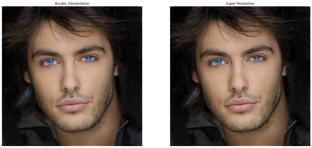
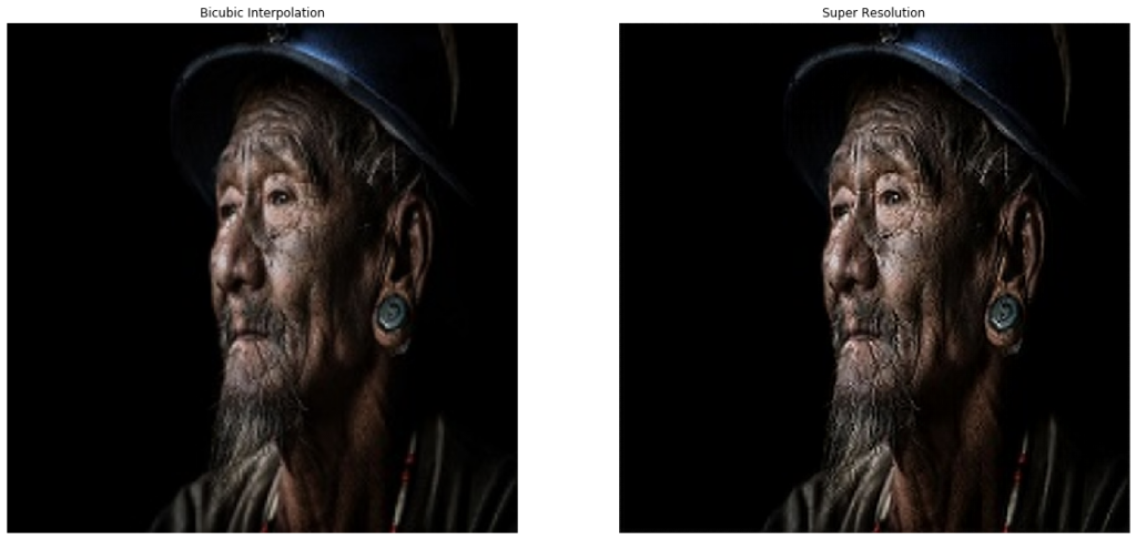
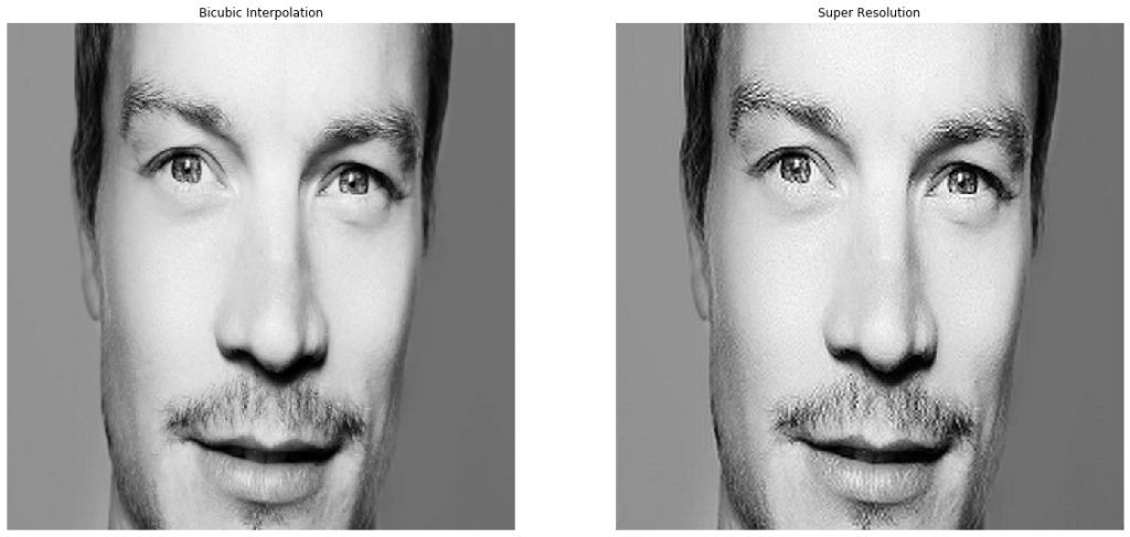
Now pass in any image to the main function and you’ll see a comparison of both its Bicubic and super-resolution version.
Granted the results are not that astonishing, it’s only doing 3x and there are models that can do 8x or more. But its a starting point, its really fast, easily under 100 ms on a CPU. And it’s better than Bicubic interpolation. And most importantly you can use this directly in OpenCV. In future I may consider writing a tutorial on other Super Resolution networks but for that I may have to use Pytorch or Tensorflow.
Applications:
Super Resolution has some great applications.
Facial Recognition: Super res algorithms can help in improving the accuracy of those Surveillance systems which have to perform facial recognition on low-resolution cameras. You can try this experiment yourself and see if this network helps you to improve performance on your facial recognition systems.
Satellite Imagery: All those satellite images can be further zoomed in without any loss in quality and with no extra hardware by just implementing super-resolution on them.
Medical: It can also prove really effective in medical imaging. Especially those images for which you are limited by the available lenses.
Data Compression/Bandwidth saving: Imagine the bandwidth savings if you can download low res images and then view in high resolution using a mobile version of a super-resolution algorithm.
In Fact if you think about it, this technique has limitless applications across many industries.
Note: There is still no Generic Super-resolution algorithm that does well in all problem domains. Meaning if you take a Super res network that was trained on a dataset of house pictures and test it on animals then it would do poorly. So almost all Super res networks have their weaknesses. The best thing is to train a super res on your own problem and then use it. The best part about it is that generating labels for any image is as easy as downsizing an image literally.
You’ll come across many Computer Vision courses out there, but nothing beats a 1 on 1 video call support from an expert in the field. Plus there is a plethora of subfields and tons of courses on AI and computer vision out there, you need someone to lay out a step-by-step learning path customized to your needs. This is where I come in, whether you need monthly support or just want to have a one-time chat with me, I’ve got you covered. Check all the coaching details and packages here
So let’s quickly Summarize what we did here, first, we discussed what is Super-resolution then we went over a series of Super Res networks and we saw how each algorithm improved over the other. We also discussed other areas of Super-Resolution like multi-image Super-resolution and domain-specific super res networks.
After that, we learned how to perform a step by step pipeline to do inference with a super res network inside the OpenCV DNN module.
I hope you enjoyed this tutorial. If you have any questions regarding this post then please feel free to comment below and I’ll gladly answer them.
You can reach out to me personally for a 1 on 1 consultation session in AI/computer vision regarding your project. Our talented team of vision engineers will help you every step of the way. Get on a call with me directlyhere.
Ready to seriously dive into State of the Art AI & Computer Vision? Then Sign up for these premium Courses by Bleed AI