Watch the Full Video Here:

So far in our Contour Detection 101 series, we have made significant progress unpacking many of the techniques and tools that you will need to build useful vision applications. In part 1, we learned the basics, how to detect and draw the contours, in part 2 we learned to do some contour manipulations.

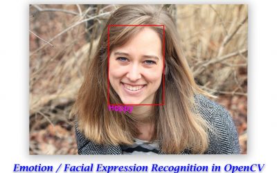
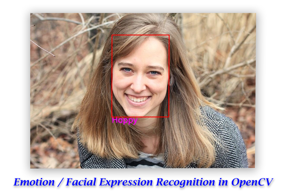
Now in the third part of this series, we will be learning about analyzing contours. This is really important because by doing contour analysis you can actually recognize the object being detected and differentiate one contour from another. We will also explore how you can identify different properties of contours to retrieve useful information. Once you start analyzing the contours, you can do all sorts of cool things with them. The application below that I made, uses contour analysis to detect the shapes being drawn!

You can build this too! In fact, I have an entire course that will help you master contours for building computer vision applications, where you learn by building all sorts of cool vision applications!

This post will be the third part of the Contour Detection 101 series. All 4 posts in the series are titled as:

1. Contour Detection 101: The Basics  
2. Contour Detection 101: Contour Manipulation
3. Contour Detection 101: Contour Analysis (This Post) 
4. Vehicle Detection with OpenCV using Contours + Background Subtraction

So if you haven’t seen any of the previous posts make sure you do check them out since in this part we are going to build upon what we have learned before so it will be helpful to have the basics straightened out if you are new to contour detection.

Alright, now we can get started with the Code.

Download Code

[optin-monster slug=”lrrdqnjzfuycvuetarn2″]

Import the Libraries

Let’s start by importing the required libraries.

import cv2
import math
import numpy as np
import pandas as pd
import transformations
import matplotlib.pyplot as plt

Read an Image

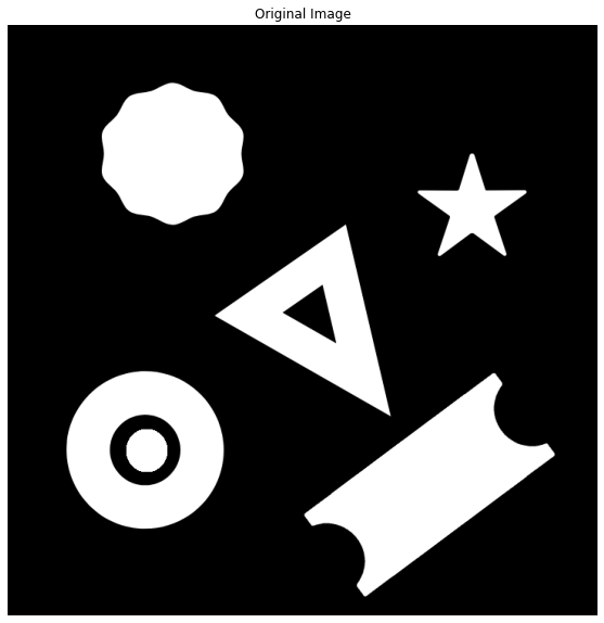
Next, let’s read an image containing a bunch of shapes.

# Read the image
image1 = cv2.imread('media/image.png') 

# Display the image
plt.figure(figsize=[10,10])
plt.imshow(image1[:,:,::-1]);plt.title("Original Image");plt.axis("off");

Detect and draw Contours

Next, we will detect and draw external contours on the image using cv2.findContours() and cv2.drawContours() functions that we have also discussed thoroughly in the previous posts.

image1_copy = image1.copy()

# Convert to grayscale
gray_scale = cv2.cvtColor(image1_copy,cv2.COLOR_BGR2GRAY)

# Find all contours in the image
contours, hierarchy = cv2.findContours(gray_scale, cv2.RETR_EXTERNAL, cv2.CHAIN_APPROX_NONE)

# Draw all the contours.
contour_image = cv2.drawContours(image1_copy, contours, -1, (0,255,0), 3);

# Display the results.
plt.figure(figsize=[10,10])
plt.imshow(contour_image[:,:,::-1]);plt.title("Image Contours");plt.axis("off");

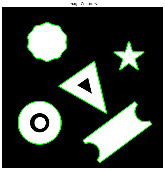
The result is a list of detected contours that can now be further analyzed for their properties. These properties are going to prove to be really useful when we build a vision application using contours. We will use them to provide us with valuable information about an object in the image and distinguish it from the other objects.

Below we will look at how you can retrieve some of these properties.

Image Moments

Image moments are like the weighted average of the pixel intensities in the image. They help calculate some features like the center of mass of the object, area of the object, etc. Finding image moments is a simple process in OpenCV which we can get by using the function cv2.moments() that returns a dictionary of various properties to use.

Function Syntax:

retval = cv.moments(array)

Parameters:

• array – Single-channel, 8-bit or floating-point 2D array

Returns:

• retval – A python dictionary containing different moments properties

# Select a contour
contour = contours[1]

# get its moments
M = cv2.moments(contour)

# print all the moments
print(M)

{‘m00’: 28977.5, ‘m10’: 4850112.666666666, ‘m01’: 15004570.666666666, ‘m20’: 878549048.4166666, ‘m11’: 2511467783.458333, ‘m02’: 7836261882.75, ‘m30’: 169397190630.30002, ‘m21’: 454938259986.68335, ‘m12’: 1311672140996.85, ‘m03’: 4126888029899.3003, ‘mu20’: 66760837.58548939, ‘mu11’: 75901.88486719131, ‘mu02’: 66884231.43453884, ‘mu30’: 1727390.3746643066, ‘mu21’: -487196.02967071533, ‘mu12’: -1770390.7230567932, ‘mu03’: 495214.8310546875, ‘nu20’: 0.07950600793808808, ‘nu11’: 9.03921532296414e-05, ‘nu02’: 0.07965295864597088, ‘nu30’: 1.2084764986041665e-05, ‘nu21’: -3.408407043976586e-06, ‘nu12’: -1.238559397771768e-05, ‘nu03’: 3.4645063088656135e-06}

The values returned represent different kinds of image movements including raw moments, central moments, scale/rotation invariant moments, and so on.

For more information on image moments and how they are calculated, you can read this Wikipedia article. Below we will discuss how some of the image moments can be used to analyze the contours detected.

Find the center of a contour

Let’s start by finding the centroid of the object in the image using the contour’s image moments. The X and Y coordinates of the Centroid are given by two relations of the central image moments, Cx=M10/M00 and Cy=M01/M00.

# Calculate the X-coordinate of the centroid
cx = int(M['m10'] / M['m00'])

# Calculate the Y-coordinate of the centroid
cy = int(M['m01'] / M['m00'])

# Print the centroid point
print('Centroid: ({},{})'.format(cx,cy))

Centroid: (167,517)

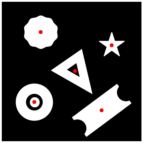
Let’s repeat the process for the rest of the contours detected and draw a circle using cv2.circle() to indicate the centroids on the image.

image1_copy = image1.copy()

# Loop over the contours
for contour in contours:

    # Get the image moments for the contour
    M = cv2.moments(contour)
    
    # Calculate the centroid
    cx = int(M['m10'] / M['m00'])
    cy = int(M['m01'] / M['m00'])

    # Draw a circle to indicate the contour
    cv2.circle(image1_copy,(cx,cy), 10, (0,0,255), -1)

# Display the results
plt.figure(figsize=[10,10])
plt.imshow(image1_copy[:,:,::-1]);plt.axis("off");

Finding Contour Area

We are already familiar with one way of finding the area of contour in the last post, using function cv2.contourArea().

# Select a contour
contour = contours[1]

# Get the area of the selected contour
area_method1 = cv2.contourArea(contour)

print('Area:',area_method1)

Area: 28977.5

Additionally, you can also find the area using the m00 moment of the contour which contains the contour’s area.

# get selected contour moments
M = cv2.moments(contour)

# Get the moment containing the Area
area_method2 = M['m00']

print('Area:',area_method2)

Area: 28977.5

As you can see, both of the methods give the same result.

Contour Properties

When building an application using contours, information about the properties of a contour is vital. These properties are often invariant to one or more transformations such as translation, scaling, and rotation. Below, we will have a look at some of these properties.

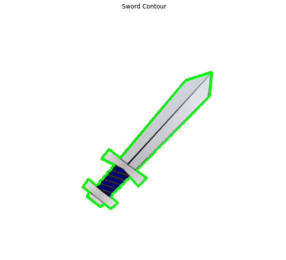
Let’s start by detecting the external contours of an image.

# Read the image
image4 = cv2.imread('media/sword.jpg') 

# Create a copy 
image4_copy = image4.copy()

# Convert to gray-scale
imageGray = cv2.cvtColor(image4_copy,cv2.COLOR_BGR2GRAY)

# create a binary thresholded image
_, binary = cv2.threshold(imageGray, 220, 255, cv2.THRESH_BINARY_INV)

# Detect and draw external contour
contours, hierarchy = cv2.findContours(binary, cv2.RETR_EXTERNAL, cv2.CHAIN_APPROX_NONE)

# Select a contour
contour = contours[0]

# Draw the selected contour
cv2.drawContours(image4_copy, contour, -1, (0,255,0), 3)

# Display the result
plt.figure(figsize=[10,10])
plt.imshow(image4_copy[:,:,::-1]);plt.title("Sword Contour");plt.axis("off");

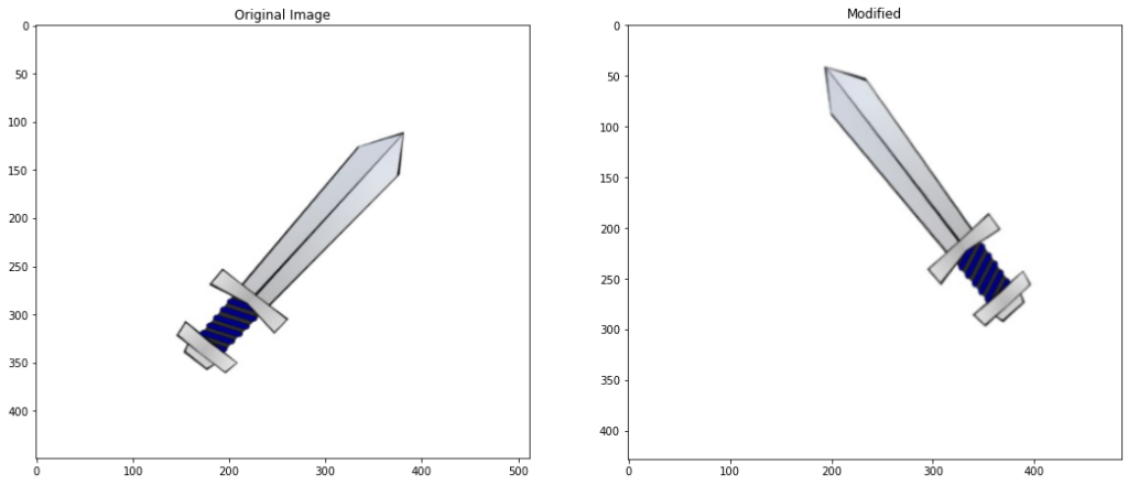
Now using a custom transform() function from the transformation.py module which you will find included with the code for this post, we can conveniently apply and display different transformations to an image.

Function Syntax:

transformations.transform(translate=True, scale=False, rotate=False, path='media/sword.jpg', display=True)

By default, only translation is applied but you may scale and rotate the image as well.

modified_contour = transformations.transform(rotate = True,scale=True)

Applied Translation of x: 44, y: 30
Applied rotation of angle: 80
Image resized to: 95.0

Aspect ratio

Aspect ratio is the ratio of width to height of the bounding rectangle of an object. It can be calculated as AR=width/height. This value is always invariant to translation.

# Get the up-right bounding rectangle for the image
x,y,w,h = cv2.boundingRect(contour)

# calculate the aspect ratio
aspect_ratio = float(w)/h
print("Aspect ratio intitially {}".format(aspect_ratio))

# Apply translation to the image and get its detected contour
modified_contour = transformations.transform(translate=True)

# Get the bounding rectangle for the detected contour
x,y,w,h = cv2.boundingRect(modified_contour)

# Calculate the aspect ratio for the modified contour
aspect_ratio = float(w)/h
print("Aspect ratio After Modification {}".format(aspect_ratio))

Aspect ratio initially 0.9442231075697212
Applied Translation of x: -45 , y: -49
Aspect ratio After Modification 0.9442231075697212

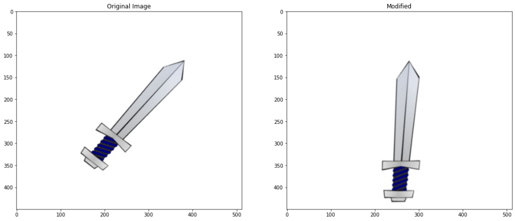
Extent 

Another useful property is the extent of a contour which is the ratio of contour area to its bounding rectangle area. Extent is invariant to Translation & Scaling.

To find the extend we start by calculating the contour area for the selected contour using the function cv2.contourArea(). Next, the bounding rectangle is found using cv2.boundingRect(). The area of the bounding rectangle is calculated using rectarea=width×height. Finally, the extent is then calculated as extent=contourarea/rectarea.

# Calculate the area for the contour
original_area = cv2.contourArea(contour)

# find the bounding rectangle for the contour
x,y,w,h = cv2.boundingRect(contour)

# calculate the area for the bounding rectangle
rect_area = w*h

# calcuate the extent
extent = float(original_area)/rect_area
print("Extent intitially {}".format(extent))

# apply scaling and translation to the image and get the contour
modified_contour = transformations.transform(translate=True,scale = True)

# Get the area of modified contour
modified_area = cv2.contourArea(modified_contour)

# Get the bounding rectangle
x,y,w,h = cv2.boundingRect(modified_contour)

# Calculate the area for the bounding rectangle
modified_rect_area = w*h

# calcuate the extent
extent = float(modified_area)/modified_rect_area

print("Extent After Modification {}".format(extent))

Extent intitially 0.2404054667406324
Applied Translation of x: 38 , y: 44
Image resized to: 117.0%
Extent After Modification 0.24218788234718347

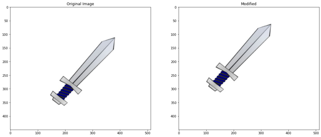
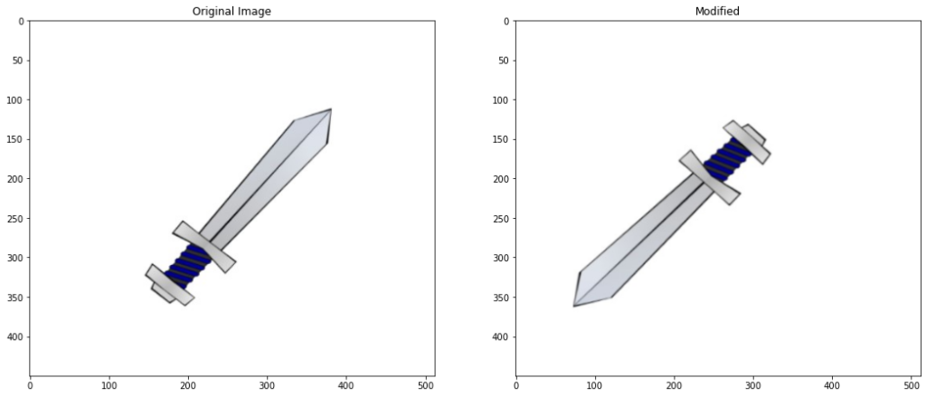
Equivalent Diameter 

Equivalent Diameter is the diameter of the circle whose area is the same as the contour area. It is Invariant to Translation & Rotation. The equivalent diameter can be calculated by first getting the area of contour with cv2.boundingRect(), the area of the circle is given by area=2×π×d²/4 where d is the diameter of the circle.

So to find the diameter we just have to make d the subject in the above equation, giving us: d=  √(4×rectArea/π).

# Calculate the diameter
equi_diameter = np.sqrt(4*original_area/np.pi)
print("Equi diameter intitially {}".format(equi_diameter))

# Apply rotation and transformation
modified_contour = transformations.transform(rotate= True)

# Get the area of modified contour
modified_area = cv2.contourArea(modified_contour)

# Calculate the diameter
equi_diameter = np.sqrt(4*modified_area/np.pi)
print("Equi diameter After Modification {}".format(equi_diameter))

Equi diameter intitially 134.93924087995146
Applied Translation of x: -39 , y: 38
Applied rotation of angle: 38
Equi diameter After Modification 135.06184863765444

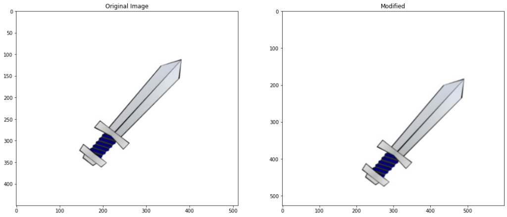
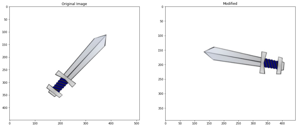
Orientation 

Orientation is simply the angle at which an object is rotated.

# Rotate and translate the contour
modified_contour = transformations.transform(translate=True,rotate= True,display = True)

Applied Translation of x: 48 , y: -37
Applied rotation of angle: 176

Now Let’s take a look at an elliptical angle on the sword contour above

# Fit and ellipse onto the contour similarly to minimum area rectangle
(x,y),(MA,ma),angle = cv2.fitEllipse(modified_contour)

# Print the angle of rotation of ellipse
print("Elliptical Angle is {}".format(angle))

Elliptical Angle is 46.882904052734375

Below method also gives the angle of the contour by fitting a rotated box instead of an ellipse

(x,y),(w,mh),angle = cv2.minAreaRect(modified_contour)
print("RotatedRect Angle is {}".format(angle))

RotatedRect Angle is 45.0

Note: Don’t be confused by why all three angles are showing different results, they all calculate angles differently, for e.g ellipse fits an ellipse and then calculates the angle that an ellipse makes, similarly the rotated rectangle calculates the angle the rectangle makes. For triggering decisions based on the calculated angle you would first need to find what angle the respective method is making at the given orientations of the object.

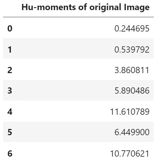
Hu moments

Hu moments are a set of 7 numbers calculated using the central moments. What makes these 7 moments special is the fact that out of these 7 moments, the first 6 of the Hu moments are invariant to translation, scaling, rotation and reflection. The 7th Hu moment is also invariant to these transformations, except that it changes its sign in case of reflection. Below we will calculate the Hu moments for the sword contour, using the moments of the contour.

You can read this paper if you want to know more about hu-moments and how they are calculated.

# Calculate moments
M = cv2.moments(contour)

# Calculate Hu Moments
hu_M = cv2.HuMoments(M)

print(hu_M)

[[5.69251998e-01]
[2.88541572e-01]
[1.37780830e-04]
[1.28680955e-06]
[2.45025329e-12]
[3.54895392e-07]
[1.69581763e-11]]

As you can see the different hu-moments have varying ranges (e.g. compare hu-moment 1 and 7) so to make the Hu-moments more comparable with each other, we will transform them to log-scale and bring them all to the same range.

# Log scale hu moments 
for i in range(0,7):
    hu_M[i] = -1* math.copysign(1.0,  hu_M[i]) * math.log10(abs(hu_M[i]))

df = pd.DataFrame(hu_M,columns=['Hu-moments of original Image']) 
df

Next up let’s apply transformations to the image and find the Hu-moments again.

# Apply translation to the image and get its detected contour
modified_contour = transformations.transform(translate = True, scale = True, rotate = True)

Applied Translation of x: -31 , y: 48
Applied rotation of angle: 122
Image resized to: 87.0%

# Calculate moments
M_modified = cv2.moments(modified_contour)

# Calculate Hu Moments
hu_Modified = cv2.HuMoments(M_modified)

# Log scale hu moments 
for i in range(0,7):
    hu_Modified[i] = -1* math.copysign(1.0, hu_Modified[i]) * math.log10(abs(hu_Modified[i]))

df['Hu-moments of Modified Image'] = hu_Modified
df

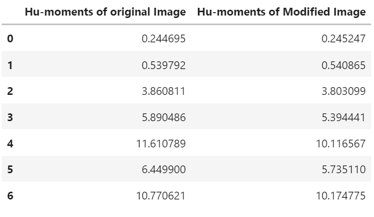
The difference is minimal because of the invariance of Hu-moments to the applied transformations.

[optin-monster slug=”d8wgq6fdm5mppdb5fi99″]

Summary

In this post, we saw how useful contour detection can be when you analyze the detected contour for its properties, enabling you to build applications capable of detecting and identifying objects in an image.

We learned how image moments can provide us useful information about a contour such as the center of a contour or the area of contour.

We also learned how to calculate different contour properties invariant to different transformations such as rotation, translation, and scaling. 

Lastly, we also explored seven unique image moments called Hu-moments which are really helpful for object detection using contours since they are invariant to translation, scaling, rotation, and reflection at once.

This concludes the third part of the series. In the next and final part of the series, we will be building a Vehicle Detection Application using many of the techniques we have learned in this series.

You can reach out to me personally for a 1 on 1 consultation session in AI/computer vision regarding your project. Our talented team of vision engineers will help you every step of the way. Get on a call with me directly here.