Watch the Full Video Here:

Let’s say you have been tasked to design a system capable of detecting vehicles on a road such as the one below,

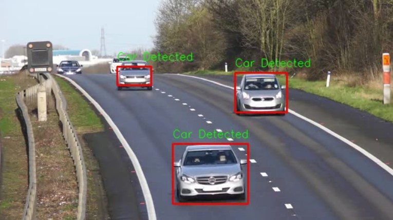
Surely, this seems like a job for a Deep Neural Network, right?

This means you have to get a lot of data, label them, then train a model, tune its performance and serve it on a system capable of running it in real-time.

This sounds like a lot of work and it begs the question: Is deep learning the only way to do so?

What if I tell you that you can solve this problem and many others like this using a much simpler approach, and with this approach, you will not have to spend days collecting data or training deep learning models. And the approach is also lightweight so it will run on almost any machine! 

Alright, what exactly are we talking about here? 

This simpler approach relies on a popular Computer Vision technique called Contour Detection. A handy technique that can save the day when dealing with vision problems such as the one above. Although not as generalizable as Deep Neural Networks, contour detection can prove robust under controlled circumstances, requiring minimum time investment and effort to build vision applications.

Just to give you a glimpse of what you can build with contour detection, have a look at some of the applications that I made using contour detection.

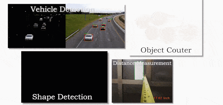
and there are many other applications that you can build too, once you learn about what contour Detection is and how you can use it, in fact, I have an entire course that will help you master contours for building computer vision applications. 

Since Contours is a lengthy topic, I’ll be breaking down Contours into a 4 parts series. This is the first part where we discuss the basics of contour detection in OpenCV, how to use it, and go over various preprocessing techniques required for Contour Detection. 

All 4 posts in the series are titled as:

1. Contour Detection 101: The Basics  (This Post)
2. Contour Detection 101: Contour Manipulation
3. Contour Detection 101: Contour Analysis 
4. Vehicle Detection with OpenCV using Contours + Background Subtraction

So without further Ado, let’s start.

Download Code

[optin-monster slug=”hbnbuvpninpsjikvs49o”]

What is a Contour?

A contour can be simply defined as a curve that joins a set of points enclosing an area having the same color or intensity. This area of uniform color or intensity forms the object that we are trying to detect, and the curve enclosing this area is the contour representing the shape of the object. So essentially, contour detection works similarly to edge-detection but with the restriction that the edges detected must form a closed path.

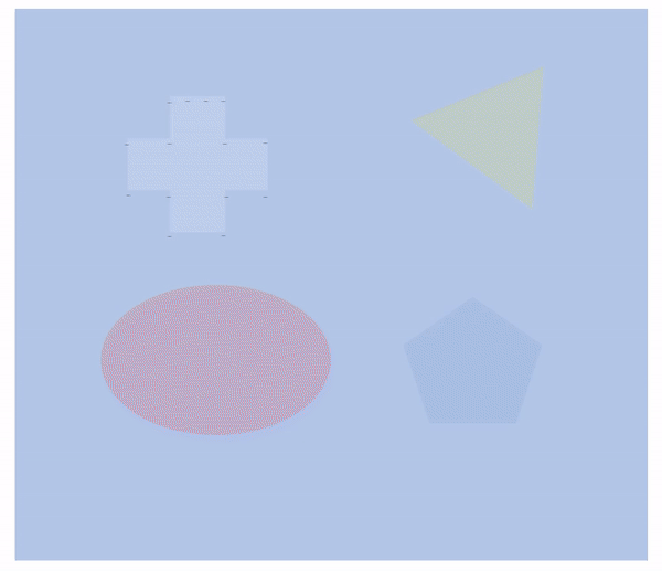
Still confused? Just have a look at the GIF below. You can see four shapes, which on a pixel level forms when certain pixels share the same color which is distinct from the background color. Contour detection identifies each of the border pixels that is distinct from the background forming an enclosed, continuous path of pixels that form the line representing the contour.

Now, let’s see how this works in OpenCV.

Import the Libraries

Let’s start by importing the required libraries.

import cv2
import numpy as np
import matplotlib.pyplot as plt

Read an Image

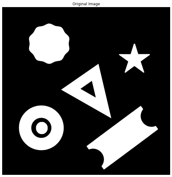
Next, we will read an image below containing a bunch of shapes for which we will find the contours.

# Read the image
Gray_image = cv2.imread('media/image.png', 0) 
 
# Display the image
plt.figure(figsize=[10,10])
plt.imshow(image1, cmap='gray');plt.title("Original Image");plt.axis("off");

OpenCV saves us the trouble of writing lengthy algorithms for contour detection and provides a handy function findContours() that analyzes the topological structure of the binary image by border following, a contour detection technique developed in 1985.

The findContours() function takes a binary image as input. The foreground is assumed to be white, and the background is assumed to be black. If that is not the case, then you can invert the image pixels using the cv2.bitwise_not() function.

Function Syntax:

contours, hierarchy = cv2.findContours(image, mode, method, contours, hierarchy, offset)

Parameters:

• image – It is the input image (8-bit single-channel). Non-zero pixels are treated as 1’s. Zero pixels remain 0’s, so the image is treated as binary. You can use compare, inRange, threshold, adaptiveThreshold, Canny, and others to create a binary image out of a grayscale or color one.
• mode – It is the contour retrieval mode, ( RETR_EXTERNAL, RETR_LIST, RETR_CCOMP, RETR_TREE )
• method – It is the contour approximation method. ( CHAIN_APPROX_NONE, CHAIN_APPROX_SIMPLE, CHAIN_APPROX_TC89_L1, etc )
• offset – It is the optional offset by which every contour point is shifted. This is useful if the contours are extracted from the image ROI, and then they should be analyzed in the whole image context.

Returns:

• contours – It is the detected contours. Each contour is stored as a vector of points.
• hierarchy – It is the optional output vector containing information about the image topology. It has been described in detail in the video above.

We will go through all the important parameters in a while. For now, let’s detect some contours in the image that we read above.

Since the image read above only contains a single channel instead of three, and even that channel is in the binary state (black & white) so it can be directly passed to the findContours() function without requiring any preprocessing.

# Find all contours in the image.
contours, hierarchy = cv2.findContours(Gray_image, cv2.RETR_EXTERNAL, cv2.CHAIN_APPROX_SIMPLE)

# Display the total number of contours found.
print("Number of contours found = {}".format(len(contours)))

Number of contours found = 5

Visualizing the Contours detected

As you can see the cv2.findContours() function was able to correctly detect the 5 external shapes in the image. But how do we know that the detections were correct? Thankfully we can easily visualize the detected contours using the cv2.drawContours() function which simply draws the detected contours onto an image.

Function Syntax:

cv2.drawContours(image, contours, contourIdx, color, thickness, lineType, hierarchy, maxLevel, offset)

Parameters:

• image – It is the image on which contours are to be drawn.
• contours – It is point vector(s) representing the contour(s). It is usually an array of contours.
• contourIdx – It is the parameter, indicating a contour to draw. If it is negative, all the contours are drawn.
• color – It is the color of the contours.
• thickness – It is the thickness of lines the contours are drawn with. If it is negative (for example, thickness=FILLED ), the contour interiors are drawn.
• lineType – It is the type of line. You can find the possible options here.
• hierarchy – It is the optional information about hierarchy. It is only needed if you want to draw only some of the contours (see maxLevel ).
• maxLevel – It is the maximal level for drawn contours. If it is 0, only the specified contour is drawn. If it is 1, the function draws the contour(s) and all the nested contours. If it is 2, the function draws the contours, all the nested contours, all the nested-to-nested contours, and so on. This parameter is only taken into account when there is a hierarchy available.
• offset – It is the optional contour shift parameter. Shift all the drawn contours by the specified offset=(dx, dy).

Let’s see how it works.

# Read the image in color mode for drawing purposes.
image1 = cv2.imread('media/image.png')  

# Make a copy of the source image.
image1_copy = image1.copy()

# Draw all the contours.
cv2.drawContours(image1_copy, contours, -1, (0,255,0), 3)

# Display the result
plt.figure(figsize=[10,10])
plt.imshow(image1_copy[:,:,::-1]);plt.axis("off");

This seems to have worked nicely. But again, this is a pre-processed image that is easy to work with, which will not be the case when working with a real-world problem where you will have to pre-process the image before detecting contours. So let’s have a look at some common pre-processing techniques below.

Pre-processing images For Contour Detection

As you have seen above that the cv2.findContours() functions takes in as input a single channel binary image, however, in most cases the original image will not be a binary image. Detecting contours in colored images require pre-processing to produce a single-channel binary image that can be then used for contour detection. Ideally, this processed image should have the target objects in the foreground.

The two most commonly used techniques for this pre-processing are:

• Thresholding based Pre-processing
• Edge Based Pre-processing

Below we will see how you can accurately detect contours using these techniques.

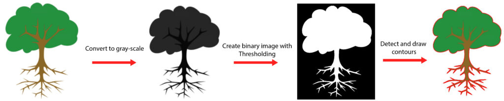
Thresholding based Pre-processing For Contours

So to detect contours in colored images we can perform fixed level image thresholding to produce a binary image, that can be then used for contour detection. Let’s see how this works.

First, read a sample image using the function cv2.imread() and display the image using the matplotlib library.

# Read the image
image2 = cv2.imread('media/tree.jpg') 

# Display the image
plt.figure(figsize=[10,10])
plt.imshow(image2[:,:,::-1]);plt.title("Original Image");plt.axis("off");

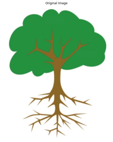
We will try to find the contour for the tree above, first without using any thresholding to see how the result will look like.

The first step is to convert the 3-channel BGR image to a single-channel image using the cv2.cvtColor() function.

# Make a copy of the source image.
image2_copy = image2.copy()

# Convert the image to gray-scale
gray = cv2.cvtColor(image2_copy, cv2.COLOR_BGR2GRAY)

# Display the result
plt.imshow(gray, cmap="gray");plt.title("Gray-scale Image");plt.axis("off");

Contour detection on the image above will only result in a contour outlining the edges of the image. This is because the cv2.findContours() function expects the foreground to be white, and the background to be black, which is not the case above so we need to invert the colors using cv2.bitwise_not().

# Invert the colours
gray_inverted = cv2.bitwise_not(gray)

# Display the result
plt.figure(figsize=[10,10])
plt.imshow(gray_inverted ,cmap="gray");plt.title("Bitwise Inverted");plt.axis("off");

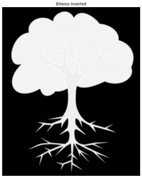
The inverted image with a black background and white foreground can now be used for contour detection.

# Find the contours from the inverted gray-scale image
contours, hierarchy = cv2.findContours(gray_inverted, cv2.RETR_EXTERNAL, cv2.CHAIN_APPROX_NONE)

# draw all contours
cv2.drawContours(image2_copy, contours, -1, (0, 255, 0), 2)

# Display the result
plt.figure(figsize=[10,10])
plt.imshow(image2_copy[:,:,::-1]);plt.title("Contours Detected");plt.axis("off");

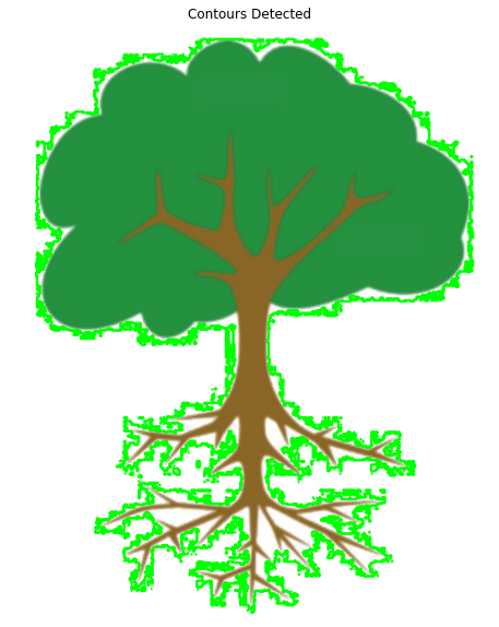
The result is far from ideal. As you can see the contours detected poorly align with the boundary of the tree in the image. This is because we only fulfilled the requirement of a single-channel image, but we did not make sure that the image was binary in colors, leaving noise along the edges. This is why we need thresholding to provide us a binary image.

Thresholding the image

We will use the function cv2.threshold() to perform thresholding. The function takes in as input the gray-scale image, applies fixed level thresholding, and returns a binary image. In this case, all the pixel values below 100 are set to 0(black) while the ones above are set to 255(white). Since the image has already been inverted, cv2.THRESH_BINARY is used, but if the image is not inverted, cv2.THRESH_BINARY_INV should be used. Also, the fixed level used must be able to correctly segment the target object as foreground(white).

# Create a binary thresholded image
_, binary = cv2.threshold(gray_inverted, 100, 255, cv2.THRESH_BINARY)

# Display the result
plt.figure(figsize=[10,10])
plt.imshow(binary, cmap="gray");plt.title("Binary Image");plt.axis("off");

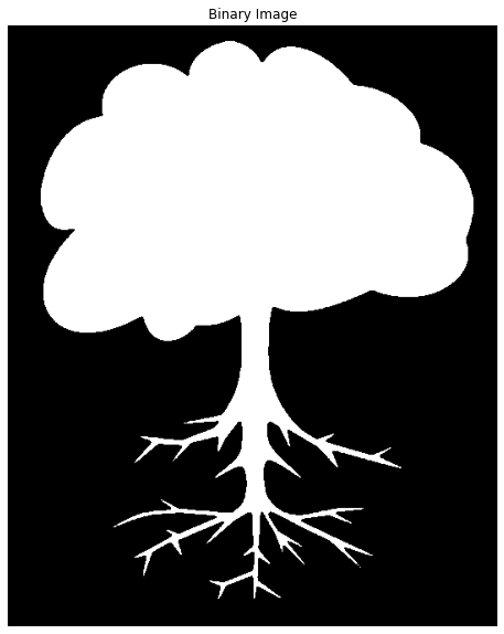
The resultant image above is ideally what the cv2.findContours() function is expecting. A single-channel binary image with Black background and white foreground.

# Make a copy of the source image.
image2_copy2 = image2.copy()

# find the contours from the thresholded image
contours, hierarchy = cv2.findContours(binary, cv2.RETR_LIST, cv2.CHAIN_APPROX_SIMPLE)

# draw all the contours found
image2_copy2 = cv2.drawContours(image2_copy2, contours, -1, (0, 0, 255), 2)

# Plot both of the resuts for comparison
plt.figure(figsize=[15,15])
plt.subplot(121);plt.imshow(image2_copy[:,:,::-1]);plt.title("Without Thresholding");plt.axis('off')
plt.subplot(122);plt.imshow(image2_copy2[:,:,::-1]);plt.title("With Threshloding");plt.axis('off');

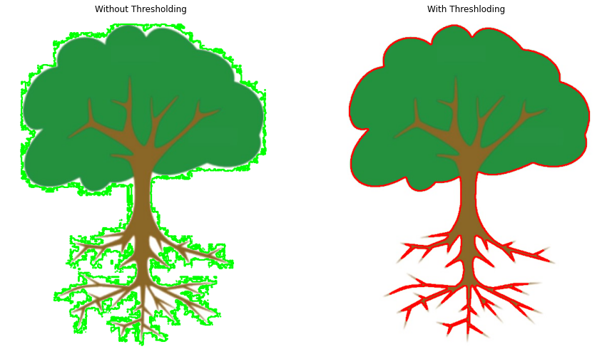
The difference is clear. Binarizing the image helps get rid of all the noise at the edges of objects, resulting in accurate contour detection.

Edge Based Pre-processing For Contours

Thresholding works well for simple images with fewer variations in colors, however, for complex images, it’s not always easy to do background-foreground segmentation using thresholding. In these cases creating the binary image using edge detection yields better results.

Let’s read another sample image.

# Read the image
image3 = cv2.imread('media/chess.jpg') 

# Display the image
plt.figure(figsize=[10,10])
plt.imshow(image3[:,:,::-1]);plt.title("Original Image");plt.axis("off");

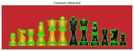
It’s obvious that simple fixed level thresholding wouldn’t work for this image. You will always end up with only half the chess pieces in the foreground only. So instead we will use the function cv2.Canny() for detecting the edges in the image. cv2.Canny() returns a single channel binary image which is all we need to perform contour detection in the next step. We also make use of the cv2.GaussianBlur() function to smoothen any noise in the image.

# Blur the image to remove noise
blurred_image = cv2.GaussianBlur(image3.copy(),(5,5),0)

# Apply canny edge detection
edges = cv2.Canny(blurred_image, 100, 160)

# Display the resultant binary image of edges
plt.figure(figsize=[10,10])
plt.imshow(edges,cmap='Greys_r');plt.title("Edges Image");plt.axis("off");

Now, using the edges detected, we can perform contour detection.

# Detect the contour using the edges
contours, hierarchy = cv2.findContours(edges, cv2.RETR_EXTERNAL, cv2.CHAIN_APPROX_SIMPLE)

# Draw the contours
image3_copy = image3.copy()
cv2.drawContours(image3_copy, contours, -1, (0, 255, 0), 2)

# Display the drawn contours
plt.figure(figsize=[10,10])
plt.imshow(image3_copy[:,:,::-1]);plt.title("Contours Detected");plt.axis("off");

In comparison, if we were to use thresholding as before it would yield a poor result that will only manage to correctly outline half of the chess pieces in the image at a time. So for a fair comparison, we will use cv2.adaptiveThreshold() to perform adaptive thresholding which adjusts to different color intensities in the image.

image3_copy2 = image3.copy()

# Remove noise from the image
blurred = cv2.GaussianBlur(image3_copy2,(3,3),0)

# Convert the image to gray-scale
gray = cv2.cvtColor(blurred, cv2.COLOR_BGR2GRAY)

# Perform adaptive thresholding 
binary = cv2.adaptiveThreshold(gray,255,cv2.ADAPTIVE_THRESH_GAUSSIAN_C,cv2.THRESH_BINARY_INV, 11, 5)

# Detect and Draw contours
contours, hierarchy = cv2.findContours(binary, cv2.RETR_EXTERNAL, cv2.CHAIN_APPROX_SIMPLE)
cv2.drawContours(image3_copy2, contours, -1, (0, 255, 0), 2)

# Plotting both results for comparison
plt.figure(figsize=[14,10])
plt.subplot(211);plt.imshow(image3_copy2[:,:,::-1]);plt.title("Using Adaptive Thresholding");plt.axis('off')
plt.subplot(212);plt.imshow(image3_copy[:,:,::-1]);plt.title("Using Edge Detection");plt.axis('off');

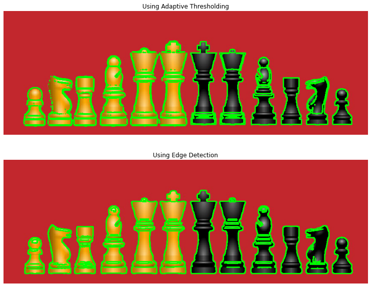
As can be seen above, using canny edge detection results in finer contour detection.

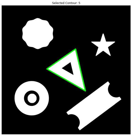
Drawing a selected Contour

So far we have only drawn all of the detected contours in an image, but what if we want to only draw certain contours?

The contours returned by the cv2.findContours() is a python list where the ith element is the contour for a certain shape in the image. Therefore if we are interested in just drawing one of the contours we can simply index it from the contours list and draw the selected contour only.

image1_copy = image1.copy()

# Find all contours in the image.
contours, hierarchy = cv2.findContours(Gray_image, cv2.RETR_LIST, cv2.CHAIN_APPROX_NONE)

# Select a contour
index = 5
contour_selected = contours[index]

# Draw the selected contour
cv2.drawContours(image1_copy, contour_selected, -1, (0,255,0), 6);

# Display the result
plt.figure(figsize=[10,10])
plt.imshow(image1_copy[:,:,::-1]);plt.axis("off");plt.title('Selected Contour: ' + str(index));

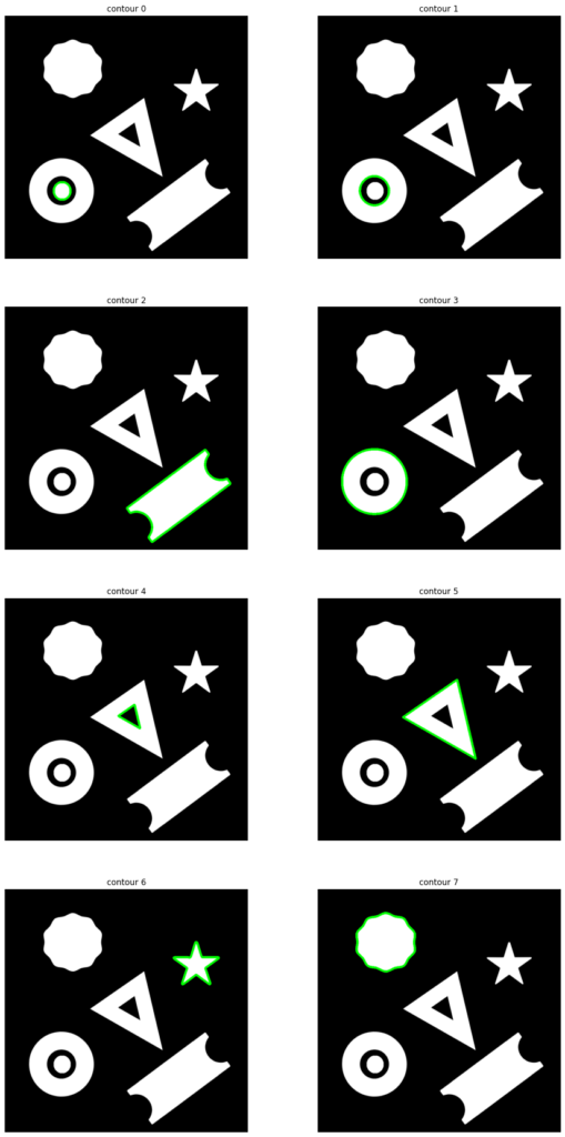
Now let’s modify our code using a for loop to draw all of the contours separately.

image1_copy = image1.copy()

# Create a figure object for displaying the images
plt.figure(figsize=[15,30])

# Convert to grayscale.
imageGray = cv2.cvtColor(image1_copy,cv2.COLOR_BGR2GRAY)

# Find all contours in the image
contours, hierarchy = cv2.findContours(imageGray, cv2.RETR_LIST, cv2.CHAIN_APPROX_NONE)

# Loop over the contours
for i,cont in enumerate(contours):
        
        # Draw the ith contour
        image1_copy = cv2.drawContours(image1.copy(), cont, -1, (0,255,0), 6)

        # Add a subplot to the figure
        plt.subplot(4, 2, i+1)  

        # Turn off the axis
        plt.axis("off");plt.title('contour ' +str(i))

        # Display the image in the subplot
        plt.imshow(image1_copy)

Retrieval Modes

Function cv2.findContours() does not only returns the contours found in an image but also returns valuable information about the hierarchy of the contours in the image. This hierarchy encodes how the contours may be arranged in the image, e.g, they may be nested within another contour. Often we are more interested in some contours than others. For example, you may only want to retrieve the external contour of an object.

Using the Retrieval Modes specified, the cv2.findContours() function can determine how the contours are to be returned or arranged in a hierarchy.

For more information on Retrieval modes and contour hierarchy Read here.

Some of the important retrieval modes are:

• cv2.RETR_EXTERNAL – retrieves only the extreme outer contours.
• cv2.RETR_LIST – retrieves all of the contours without establishing any hierarchical relationships.
• cv2.RETR_TREE – retrieves all of the contours and reconstructs a full hierarchy of nested contours.
• cv2.RETR_CCOMP – retrieves all of the contours and organizes them into a two-level hierarchy. At the top level, there are external boundaries of the components. At the second level, there are boundaries of the holes. If there is another contour inside a hole of a connected component, it is still put at the top level.

Below we will have a look at how each of these modes return the contours.

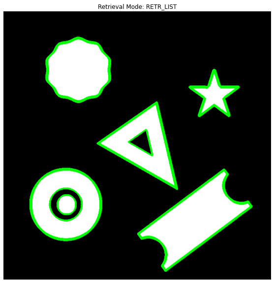
cv2.RETR_LIST

cv2.RETR_LIST simply retrieves all of the contours without establishing any hierarchical relationships between them. All of the contours can be said to have no parent or child relationship with another contour.

image1_copy = image1.copy()

# Convert to gray-scale
imageGray = cv2.cvtColor(image1_copy, cv2.COLOR_BGR2GRAY)

# Find and return all contours in the image using the RETR_LIST mode
contours, hierarchy = cv2.findContours(imageGray, cv2.RETR_LIST, cv2.CHAIN_APPROX_SIMPLE)

# Draw all contours.
cv2.drawContours(image1_copy, contours, -1, (0,255,0), 3);

# Print the number of Contours returned
print("Number of Contours Returned: {}".format(len(contours)))

# Display the results.
plt.figure(figsize=[10,10])
plt.imshow(image1_copy);plt.axis("off");plt.title('Retrieval Mode: RETR_LIST');

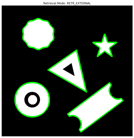
cv2.RETR_EXTERNAL

cv2.RETR_EXTERNAL retrieves only the extreme outer contours i.e the contours not having any parent contour.

image1_copy = image1.copy()

# Find all contours in the image.
contours, hierarchy = cv2.findContours(imageGray, cv2.RETR_EXTERNAL, cv2.CHAIN_APPROX_SIMPLE)

# Draw all the contours.
cv2.drawContours(image1_copy, contours, -1, (0,255,0), 3);

# Print the number of Contours returned
print("Number of Contours Returned: {}".format(len(contours)))

# Display the results.
plt.figure(figsize=[10,10])
plt.imshow(image1_copy);plt.axis("off");plt.title('Retrieval Mode: RETR_EXTERNAL');

Number of Contours Returned: 5

cv2.RETR_TREE

cv2.RETR_TREE retrieves all of the contours and constructs a full hierarchy of nested contours.

src_copy = image1.copy()

# Convert to gray-scale
imageGray = cv2.cvtColor(src_copy,cv2.COLOR_BGR2GRAY)

# Find all contours in the image while maintaining a hierarchy
contours, hierarchy = cv2.findContours(imageGray, cv2.RETR_TREE, cv2.CHAIN_APPROX_SIMPLE)

# Draw all the contours.
contour_image = cv2.drawContours(src_copy, contours, -1, (0,255,0), 3);

# Print the number of Contours returned
print("Number of Contours Returned: {}".format(len(contours)))

# Display the results.
plt.figure(figsize=[10,10])
plt.imshow(contour_image);plt.axis("off");plt.title('Retrieval Mode: RETR_TREE');

Number of Contours Returned: 8

cv2.RETR_CCOMP

cv2.RETR_CCOMP retrieves all of the contours and organizes them into a two-level hierarchy. At the top level, there are external boundaries of the object. At the second level, there are boundaries of the holes in object. If there is another contour inside that hole, it is still put at the top level.

To visualize the two levels we check for the contours that do not have any parent i.e the fourth value in their hierarchy [Next, Previous, First_Child, Parent] is set to -1. These contours form the first level and are represented with green color while all other are second-level contours represented in red.

src_copy = image1.copy()
imageGray = cv2.cvtColor(src_copy,cv2.COLOR_BGR2GRAY)

# Find all contours in the image using RETE_CCOMP method 
contours, hierarchy = cv2.findContours(imageGray, cv2.RETR_CCOMP, cv2.CHAIN_APPROX_NONE)

# Loop over all the contours detected
for i,cont in enumerate(contours):
    
    # If the contour is at first level draw it in green 
    if hierarchy[0][i][3] == -1:
        src_copy = cv2.drawContours(src_copy, cont, -1, (0,255,0), 3)
        
    # else draw the contour in Red
    else:
        src_copy = cv2.drawContours(src_copy, cont, -1, (255,0,0), 3)

# Print the number of Contours returned
print("Number of Contours Returned: {}".format(len(contours)))

# Display the results.
plt.figure(figsize=[10,10])
plt.imshow(src_copy);plt.axis("off");plt.title('Retrieval Mode: RETR_CCOMP');

Number of Contours Returned: 8

[optin-monster slug=”d8wgq6fdm5mppdb5fi99″]

Summary

Alright, In the first part of the series we have unpacked a lot of important things about contour detection and how it works. We discussed what types of applications you can build using Contour Detection and the circumstances under which it works most effectively.

We saw how you can effectively detect contours and visualize them too using OpenCV.

The post also went over some of the most common pre-processing techniques used prior to contour detection.

• Thresholding based Pre-processing
• Edge Based Pre-processing

which will help you get accurate results with contour detection. But these are not the only contour detection techniques, ultimately, it depends on what type of problem you are trying to solve, and figuring out the appropriate pre-processing to use is the key to contour detection. Start by asking what properties distinguish the target object from the rest of the image? Then figure out the best way you can use to isolate those properties.

We also went over the important Retrieval Modes that can be used to change how the hierarchy of the detected contours works or even change what type of contours are detected. Additionally, you can always use the hierarchy to only extract the contours you want, e.g. retrieve only the contours at level three.

This was the first part of the series but there are four more to come in which we will dive deeper into contour detection with OpenCV and also build a cool vision application using contour Detection!

You can reach out to me personally for a 1 on 1 consultation session in AI/computer vision regarding your project. Our talented team of vision engineers will help you every step of the way. Get on a call with me directly here.