In the previous post of this series, we introduced you to contour detection, a popular computer vision technique that you must have in your bag of tricks when dealing with computer vision problems. We discussed how we can detect contours for an object in an image, the pre-processing steps involved to prepare the image for contour detection, and we also went over many of the useful retrieval modes that you can use when detecting contours.
But detecting and drawing contours alone won’t cut it if you want to build powerful computer vision applications. Once detected, the contours need to be processed to make them useful for building cool applications such as the one below.
This is why in this second part of the series we will learn how we can perform different contour manipulations to extract useful information from the detected contours. Using this information you can build application such as the one above and many others, once you learn about how to effectively use and manipulate contours, in fact, I have an entire course that will help you master contours for building computer vision applications.
This post will be the second part of our new Contour Detection 101 series. All 4 posts in the series are titled as:
So if you haven’t seen the previous post and you are new to contour detection make sure you do check it out.
In part two of the series, the contour manipulation techniques we are going to learn will enable us to perform some important tasks such as extracting the largest contour in an image, sorting contours in terms of size, extracting bounding box regions of a targeted contour, etc. These techniques also form the building blocks for building robust classical vision applications.
So without further Ado, let’s get started.
[optin-monster slug=”sidmzfsvlmvh8o3kc5c1″]
Import the Libraries
Let’s start by importing the required libraries.
import cv2
import numpy as np
import matplotlib.pyplot as plt
Read an Image
# Read the image
image1 = cv2.imread('media/image.png')

# Display the image
plt.figure(figsize=[10,10])
plt.imshow(image1[:,:,::-1]);plt.title("Original Image");plt.axis("off");
Detect and draw Contours
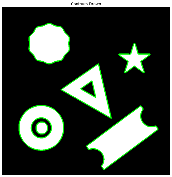
Next, we will detect and draw contours on the image as before using the cv2.findContours()andcv2.drawContours()functions.
# Make a copy of the original image so it is not overwritten
image1_copy = image1.copy()

# Convert to grayscale.
image_gray = cv2.cvtColor(image1_copy,cv2.COLOR_BGR2GRAY)

# Find all contours in the image.
contours, hierarchy = cv2.findContours(image_gray, cv2.RETR_CCOMP, cv2.CHAIN_APPROX_NONE)

# Draw the selected contour
cv2.drawContours(image1_copy, contours, -1, (0,255,0), 3);

# Display the result
plt.figure(figsize=[10,10])
plt.imshow(image1_copy[:,:,::-1]);plt.axis("off");plt.title('Contours Drawn');
Extracting the Largest Contour in the image
When building vision applications using contours, often we are interested in retrieving the contour of the largest object in the image and discard others as noise. This can be done using the built-in python’s max() function with the contours list. The max() function takes in as input the contours list along with a key parameter which refers to the single argument function used to customize the sort order. The function is applied to each item on the iterable. So for retrieving the largest contour we use the key cv2.contourArea which is a function that returns the area of a contour. It is applied to each contour in the list and then the max() function returns the largest contour based on its area.
image1_copy = image1.copy()

# Convert to grayscale
gray_image = cv2.cvtColor(image1_copy,cv2.COLOR_BGR2GRAY)

# Find all contours in the image.
contours, hierarchy = cv2.findContours(gray_image, cv2.RETR_LIST, cv2.CHAIN_APPROX_NONE)

# Retreive the biggest contour
biggest_contour = max(contours, key = cv2.contourArea)

# Draw the biggest contour
cv2.drawContours(image1_copy, biggest_contour, -1, (0,255,0), 4);

# Display the results
plt.figure(figsize=[10,10])
plt.imshow(image1_copy[:,:,::-1]);plt.axis("off");
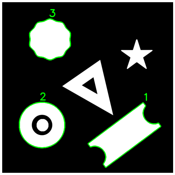
Sorting Contours in terms of size
Extracting the largest contour worked out well, but sometimes we are interested in more than one contour from a sorted list of contours. In such cases, another built-in python function sorted() can be used instead. sorted() function also takes in the optional key parameter which we use as before for returning the area of each contour. Then the contours are sorted based on area and the resultant list is returned. We also specify the order of sort reverse = True i.e in descending order of area size.
image1_copy = image1.copy()

# Convert to grayscale.
imageGray = cv2.cvtColor(image1_copy,cv2.COLOR_BGR2GRAY)

# Find all contours in the image.
contours, hierarchy = cv2.findContours(imageGray, cv2.RETR_CCOMP, cv2.CHAIN_APPROX_NONE)

# Sort the contours in decreasing order
sorted_contours = sorted(contours, key=cv2.contourArea, reverse= True)

# Draw largest 3 contours
for i, cont in enumerate(sorted_contours[:3],1):

    # Draw the contour
    cv2.drawContours(image1_copy, cont, -1, (0,255,0), 3)

    # Display the position of contour in sorted list
    cv2.putText(image1_copy, str(i), (cont[0,0,0], cont[0,0,1]-10), cv2.FONT_HERSHEY_SIMPLEX, 1.4, (0, 255, 0),4)


# Display the result
plt.figure(figsize=[10,10])
plt.imshow(image1_copy[:,:,::-1]);plt.axis("off");
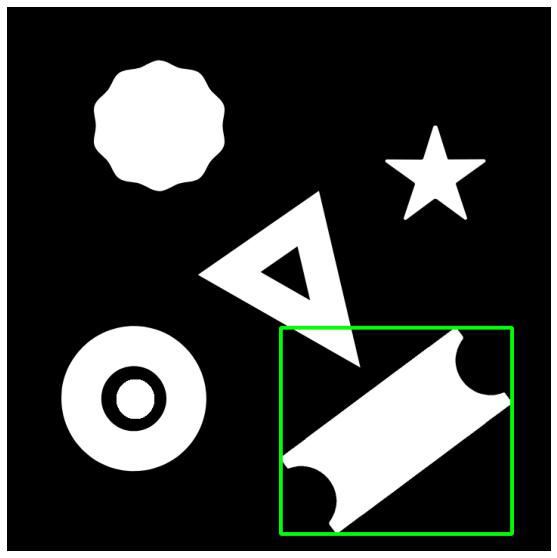
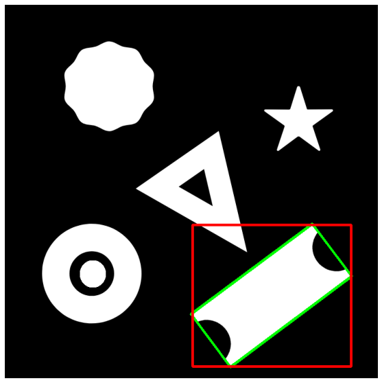
Drawing a rectangle around the contour
Bounding rectangles are often used to highlight the regions of interest in the image. If this region of interest is a detected contour of a shape in the image, we can enclose it within a rectangle. There are two types of bounding rectangles that you may draw:
Straight Bounding Rectangle
Rotated Rectangle
For both types of bounding rectangles, their vertices are calculated using the coordinates in the contour list.
Straight Bounding Rectangle
A straight bounding rectangle is simply an upright rectangle that does not take into account the rotation of the object. Its vertices can be calculated using the cv2.boundingRect() function which calculates the vertices for the minimal up-right rectangle possible using the extreme coordinates in the contour list. The coordinates can then be drawn as rectangle using cv2.rectangle() function.
array – It is the Input gray-scale image or 2D point set from which the bounding rectangle is to be created
Returns:
x – It is X-coordinate of the top-left corner
y – It is Y-coordinate of the top-left corner
w – It is the width of the rectangle
h – It is the height of the rectangle
image1_copy = image1.copy()

# Convert to grayscale.
gray_scale = cv2.cvtColor(image1_copy,cv2.COLOR_BGR2GRAY)

# Find all contours in the image.
contours, hierarchy = cv2.findContours(gray_scale, cv2.RETR_CCOMP, cv2.CHAIN_APPROX_NONE)

# Get the bounding rectangle
x, y, w, h = cv2.boundingRect(contours[1])

# Draw the rectangle around the object.
cv2.rectangle(image1_copy, (x, y), (x+w, y+h), (0, 255, 0), 3)

# Display the result
plt.figure(figsize=[10,10])
plt.imshow(image1_copy[:,:,::-1]);plt.axis("off");
However, the bounding rectangle created is not a minimum area bounding rectangle often causing it to overlap with any other objects in the image. But what if the rectangle is rotated so that the area can be minimized to tightly fit the shape.
Rotated Rectangle
As the name suggests the rectangle drawn is rotated at an angle so that the area it occupies to enclose the contour is minimum. The function you can use to calculate the vertices of the rotated rectangle is cv2.minAreaRect(), which uses the contour point set to calculate the coordinates of the top left corner of the rectangle, its width, height, and the angle of rotation of the rectangle.
array – It is the Input gray-scale image or 2D point set from which the bounding rectangle is to be created
Returns:
retval – A tuple consisting of:
x,y coordinates of the top-left vertex
width, height of the rectangle
angle of rotation of the rectangle
Since the cv2.rectangle() function can only draw up-right rectangles we cannot use it to draw the rotated rectangle. Instead, we can calculate the 4 vertices of the rectangle using the cv2.boxPoints() function which takes the rect tuple as input. Once we have the vertices, the rectangle can be simply drawn using the cv2.drawContours() function.
image1_copy = image1.copy()
# Convert to grayscale
gray_scale = cv2.cvtColor(image1_copy,cv2.COLOR_BGR2GRAY)
# Find all contours in the image
contours, hierarchy = cv2.findContours(gray_scale, cv2.RETR_CCOMP, cv2.CHAIN_APPROX_NONE)
# calculate the minimum area Bounding rect
rect = cv2.minAreaRect(contours[1])
# Check out the rect object
print(rect)
# convert the rect object to box points
box = cv2.boxPoints(rect).astype('int')
# Draw a rectangle around the object
cv2.drawContours(image1_copy,
This is the minimum area bounding rectangle possible. Let’s see how it compares to the straight bounding box.
# Draw the up-right rectangle
cv2.rectangle(image1_copy, (x, y), (x+w, y+h), (0,0, 255), 3)

# Display the result
plt.figure(figsize=[10,10])
plt.imshow(image1_copy[:,:,::-1]);plt.axis("off");
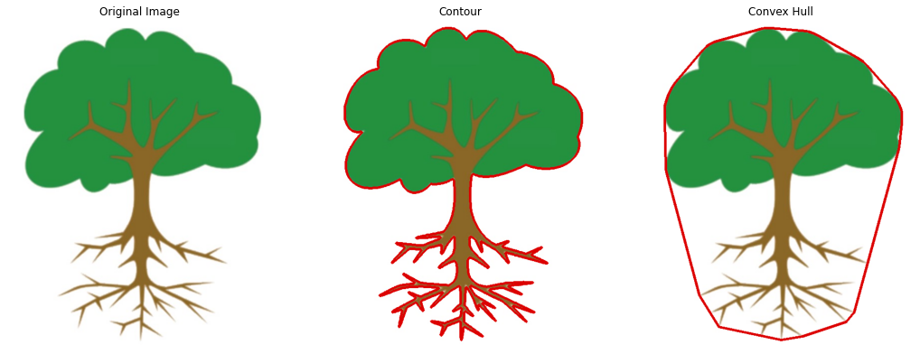
Drawing Convex Hull
A convex hull is another useful way to represent the contour onto the image. The function cv2.convexHull() checks a curve for convexity defects and corrects it. Convex curves are curves that are bulged out. And if it is bulged inside (Concave), it is called convexity defects.
Finding the convex hull of a contour can be very useful when working with shape matching techniques. This is because the convex hull of a contour highlights its prominent features while discarding smaller variations in the shape.
points – Input 2D point set. This is a single contour.
clockwise – Orientation flag. If it is true, the output convex hull is oriented clockwise. Otherwise, it is oriented counter-clockwise. The assumed coordinate system has its X axis pointing to the right, and its Y axis pointing upwards.
returnPoints – Operation flag. In case of a matrix, when the flag is true, the function returns convex hull points. Otherwise, it returns indices of the convex hull points. By default it is True.
Returns:
hull – Output convex hull. It is either an integer vector of indices or vector of points. In the first case, the hull elements are 0-based indices of the convex hull points in the original array (since the set of convex hull points is a subset of the original point set). In the second case, hull elements are the convex hull points themselves.
image2 = cv2.imread('media/tree.jpg')

hull_img = image2.copy()
contour_img = image2.copy()

# Convert the image to gray-scale
gray = cv2.cvtColor(image2, cv2.COLOR_BGR2GRAY)

# Create a binary thresholded image
_, binary = cv2.threshold(gray, 230, 255, cv2.THRESH_BINARY_INV)

# Find the contours from the thresholded image
contours, hierarchy = cv2.findContours(binary, cv2.RETR_EXTERNAL, cv2.CHAIN_APPROX_SIMPLE)

# Since the image only has one contour, grab the first contour
cnt = contours[0]

# Get the required hull
hull = cv2.convexHull(cnt)

# draw the hull
cv2.drawContours(hull_img, [hull], 0 , (0,0,220), 3)

# draw the contour
cv2.drawContours(contour_img, [cnt], 0, (0,0,220), 3)

plt.figure(figsize=[18,18])
plt.subplot(131);plt.imshow(image2[:,:,::-1]);plt.title("Original Image");plt.axis('off')
plt.subplot(132);plt.imshow(contour_img[:,:,::-1]);plt.title("Contour");plt.axis('off');
plt.subplot(133);plt.imshow(hull_img[:,:,::-1]);plt.title("Convex Hull");plt.axis('off');
[optin-monster slug=”d8wgq6fdm5mppdb5fi99″]
Summary
In today’s post, we familiarized ourselves with many of the contour manipulation techniques. These manipulations help make contour detection an even more useful tool applicable to a wider variety of problems
We saw how you can filter out contours based on their size using the built-in max() and sorted() functions, allowing you to extract the largest contour or a list of contours sorted by size.
Then we learned how you can highlight contour detections with bounding rectangles of two types, the straight bounding rectangle and the rotated one.
Lastly, we learned about convex hulls and how you can find them for detected contours. A very handy technique that can prove to be useful for object detection with shape matching.
This sums up the second post in the series. In the next post, we’re going to learn various analytical techniques to analyze contours in order to classify and distinguish between different Objects.
So if you found this lesson useful, let me know in the comments and you can also support me and the Bleed AI team on patreon here.
If you need 1 on 1 Coaching in AI/computer vision regarding your project, or your career then you reach out to mepersonally here
Hire Us
Let our team of expert engineers and managers build your next big project using Bleeding Edge AI Tools & Technologies
Did you know that you can actually stream a Live Video wirelessly from your phone’s camera to OpenCV’s cv2.VideoCapture() function in your PC and do all sorts of image processing on the spot like build an intruder detection system?
Cool huh?
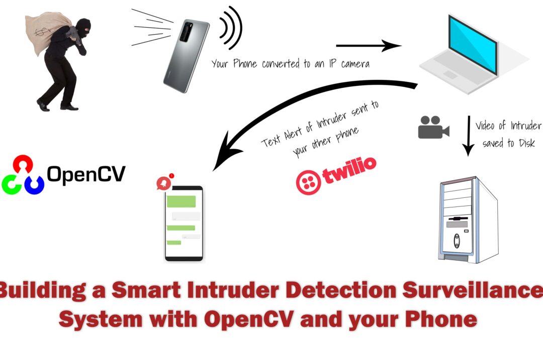
In today’s post not only we will do just that but we will also build a robust Intruder Detection surveillance system on top of that, this will record video samples whenever someone enters your room and will also send you alert messages via Twilio API.
This post will serve as your building blocks for making a smart intruder detection system with computer vision. Although I’m making this tutorial for a home surveillance experiment, you can easily take this setup and swap the mobile camera with multiple IP Cams to create a much larger system.
Today’s tutorial can be split into 4 parts:
Accessing the Live stream from your phone to OpenCV.
Learning how to use the Twilio API to send Alert messages.
Building a Motion Detector with Background Subtraction and Contour detection.
Making the Final Application
You can watch the full application demo here
So most of the people have used the cv2.videocapture() function to read from a webcam or a video recording from a disk but only a few people know how easy it is to stream a video from a URL, in most cases this URL is from an IP camera.
By the way with cv2.VideoCapture() you can also read a sequence of images, so yeah a GIF can be read by this.
So let me list out all 4 ways to use VideoCapture() class depending upon what you pass inside the function.
1. Using Live camera feed: You pass in an integer number i.e. 0,1,2 etc e.g. cap = cv2.VideoCapture(0), now you will be able to use your webcam live stream. The number depends upon how many USB cams you attach and on which port.
2.Playing a saved Video on Disk: You pass in the path to the video file e.g. cap = cv2.VideoCapture(Path_To_video).
3. Live Streaming from URL using Ip camera or similar: You can stream from a URL e.g. cap = cv2.VideoCapture( protocol://host:port/video) Note: that each video stream or IP camera feed has its own URL scheme.
4.Read a sequence of Images: You can also read sequences of images, e.g. GIF.
Part 1: Accessing the Live stream from your phone to OpenCV For The Intruder Detection System:
For those of you who have an Android phone can go ahead and install this IP Camera application from playstore.
For people that want to try a different application or those of you who want to try on their iPhone I would say that although you can follow along with this tutorial by installing a similar IP camera application on your phones but one issue that you could face is that the URL Scheme for each application would be different so you would need to figure that out, some application makes it really simple like the one I’m showing you today.
You can also use the same code I’m sharing here to work with an actual IP Camera, again the only difference will be the URL scheme, different IP Cameras have different URL schemes. For our IP Camera, the URL Scheme is: protocol://host:port/video
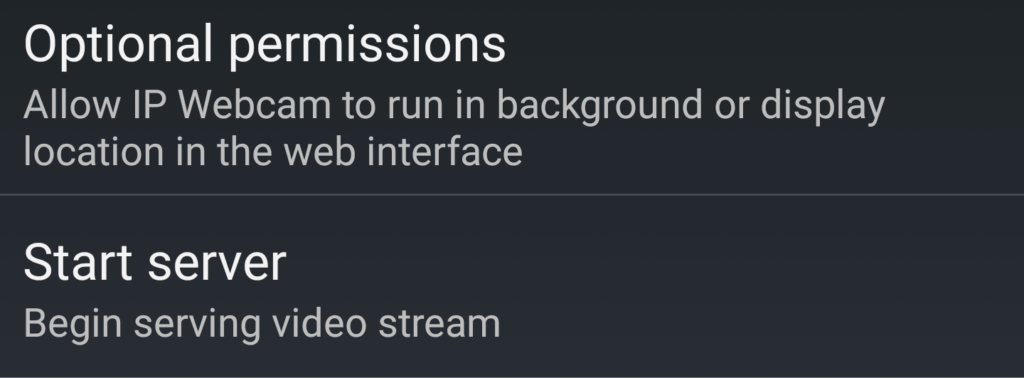
After installing the IP Camera application, open it and scroll all the way down and click start server.
After starting the server the application will start streaming the video to the highlighted URL:
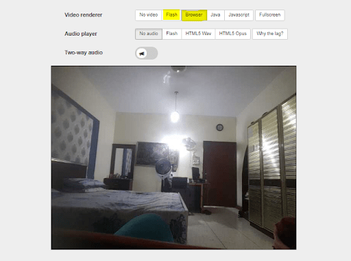
If you paste this URL in the browser of your computer then you would see this:
Note: Your computer and mobile must be connected to the same Network
Click on the Browser or the Flash button and you’ll see a live stream of your video feed:
Below the live feed, you’ll see many options on how to stream your video, you can try changing these options and see effects take place in real-time.
Some important properties to focus on are the video Quality, FPS, and the resolution of the video. All these things determine the latency of the video. You can also change front/back cameras.
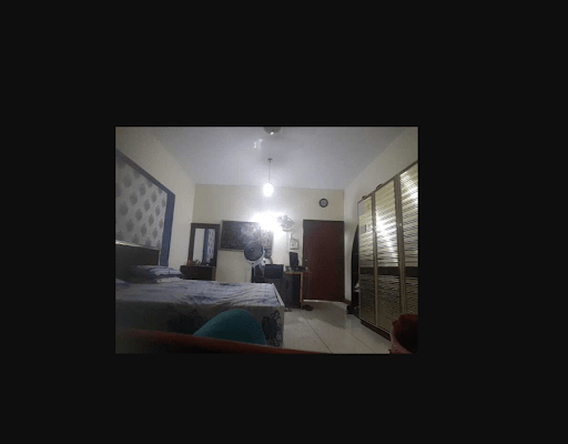
Try copying the image Address of the frame:
If you try pasting the address in a new tab then you will only see the video stream. So this is the address that will go inside the VideoCapture function.
So the URL scheme in our case is : protocol://host:port/video, where protocol is “http” , host is: “192.168.18.4” and port is: “8080”
All you have to do is paste the above address inside the VideoCapture function and you’re all set.
Download Code
[optin-monster slug=”yi4hfsyqpz8k693x41yc”]
Here’s the Full Code:
# Import the required libraries
import numpy as np
import cv2
import time
import datetime
from collections import deque
# Set Window normal so we can resize it
cv2.namedWindow('frame', cv2.WINDOW_NORMAL)

# Note the starting time
start_time = time.time()

# Initialize these variables for calculating FPS
fps = 0
frame_counter = 0

# Read the video steram from the camera
cap = cv2.VideoCapture('http://192.168.18.4:8080/video')

while(True):

    ret, frame = cap.read()
    if not ret:
        break

    # Calculate the Average FPS
    frame_counter += 1
    fps = (frame_counter / (time.time() - start_time))

    # Display the FPS
    cv2.putText(frame, 'FPS: {:.2f}'.format(fps), (20, 20), cv2.FONT_HERSHEY_SIMPLEX, 0.6, (0, 0, 255),1)

    # Show the Frame
    cv2.imshow('frame',frame)

    # Exit if q is pressed.
    if cv2.waitKey(1) == ord('q'):
        break

# Release Capture and destroy windows
cap.release()
cv2.destroyAllWindows()
As you can see I’m able to stream video from my phone.
Now there are some options you may want to consider, for e.g you may want to change the resolution, in my case I have set the resolution to be `640×480`. Since I’m not using the web interface so I have used the app to set these settings.
There are also other useful settings that you may want to do, like settings up a password and a username so your stream is protected. Setting up a password would, of course, change the URL to something like:
I’ve also enabled background mode so even when I’m out of the app or my phone screen is closed the camera is recording secretly, now this is super stealth mode.
Finally here are some other URL Schemes to read this IP Camera stream, with these URLs you can even load audio and images from the stream:
http://19412.168.3.:8080/video is the MJPEG URL.
http://192.168.43.1:8080/shot.jpg fetches the latest frame.
http://192.168.43.1:8080/audio.wav is the audio stream in Wav format.
http://192.168.43.1:8080/audio.aac is the audio stream in AAC format (if supported by hardware).
Part 2: Learning how to use the Twilio API to send Alert messages for the Intruder Detection System:
What is Twilio?
Twilio is an online service that allows us to programmatically make and receive phone calls, send and receive SMS, MMS and even Whatsapp messages, using its web APIs.
Today we’ll just be using it to send an SMS, you won’t need to purchase anything since you get some free credits after you have signed up here.
So go ahead and sign up, after signing up go to the console interface and grab these two keys and your trial Number:
ACCOUNT SID
AUTH TOKEN
After getting these keys you would need to insert them in the credentials.txt file provided in the source code folder. You can download the folder from above.
Make sure to replace the `INSERT_YOUR_ACCOUNT_SID` with your ACCOUNT SID and also replace`INSERT_YOUR_AUTH_TOKEN` with your`AUTH TOKEN.`
There are also two other things you need to insert in the text file, this is your trail Number given to by the Twilio API and your personal number where you will receive the messages.
So replace `PERSONAL_NUMBER` with your number and `TRIAL_NUMBER` with the Twilio number, make sure to include the country code for your personal number.
Note: in the trail account the personal number can’t be any random number but its verified number. After you have created the account you can add verified numbers here.
Now you’re ready to use the twilio api, you first have to install the API by doing:
pip install twilio
Now just run this code to send a message:
from twilio.rest import Client

# Read text from the credentials file and store in data variable
with open('credentials.txt', 'r') as myfile:
  data = myfile.read()

# Convert data variable into dictionary
info_dict = eval(data)

# Your Account SID from twilio.com/console
account_sid = info_dict['account_sid']

# Your Auth Token from twilio.com/console
auth_token  = info_dict['auth_token']

# Set client and send the message
client = Client(account_sid, auth_token)
message = client.messages.create( to =info_dict['your_num'], from_ = info_dict['trial_num'], body= "What's Up Man")
Check your phone you would have received a message. Later on we’ll properly fill up the body text.
Part 3: Building a Motion Detector with Background Subtraction and Contour detection:
Now in OpenCV, there are multiple ways to detect and track a moving object, but we’re going to go for a simple background subtraction method.
What are Background Subtraction methods?
Basically these kinds of methods separate the background from the foreground in a video so for e.g. if a person walks in an empty room then the background subtraction algorithm would know there’s disturbance by subtracting the previously stored image of the room (without the person ) and the current image (with the person).
So background subtraction can be used as effective motion detectors and even object counters like a people counter, how many people went in or out of a shop.
Now what I’ve described above is a very basic approach to background subtraction, In OpenCV, you would find a number of complex algorithms that use background subtraction to detect motion, In my Computer Vision & Image Processing Course I have talked about background subtraction in detail. I have taught how to construct your own custom background subtraction methods and how to use the built-in OpenCV ones. So make sure to check out the course if you want to study computer vision in depth.
For this tutorial, I will be using a Gaussian Mixture-based Background / Foreground Segmentation Algorithm. It is based on two papers by Z.Zivkovic, “Improved adaptive Gaussian mixture model for background subtraction” in 2004 and “Efficient Adaptive Density Estimation per Image Pixel for the Task of Background Subtraction” in 2006
Here’s the code to apply background subtraction:
# load a video
cap = cv2.VideoCapture('sample_video.mp4')

# Create the background subtractor object
foog = cv2.createBackgroundSubtractorMOG2( detectShadows = True, varThreshold = 50, history = 2800)

while(1):

    ret, frame = cap.read()
    if not ret:
        break

    # Apply the background object on each frame
    fgmask = foog.apply(frame)

    # Get rid of the shadows
    ret, fgmask = cv2.threshold(fgmask, 250, 255, cv2.THRESH_BINARY)

    # Show the background subtraction frame.
    cv2.imshow('All three',fgmask)
    k = cv2.waitKey(10)
    if k == 27:
        break

cap.release()
cv2.destroyAllWindows()
The `cv2.createBackgroundSubtractorMOG2()` takes in 3 arguments:
detectsSadows: Now this algorithm will also be able to detect shadows, if we pass in `detectShadows=True` argument in the constructor. The ability to detect and get rid of shadows will give us smooth and robust results. Enabling shadow detection slightly decreases speed.
history: This is the number of frames that is used to create the background model, increase this number if your target object often stops or pauses for a moment.
varThreshold: This threshold will help you filter out noise present in the frame, increase this number if there are lots of white spots in the frame. Although we will also use morphological operations like erosion to get rid of the noise.
Now after we have our background subtraction done then we can further refine the results by getting rid of the noise and enlarging our target object.
We can refine our results by using morphological operations like erosion and dilation. After we have cleaned our image then we can apply contour detection to detect those moving big white blobs (people) and then draw bounding boxes over those blobs.
If you don’t know about Morphological Operations or Contour Detection then you should go over this Computer Vision Crash course post, I published a few weeks back.
# initlize video capture object
cap = cv2.VideoCapture('sample_video.mp4')

# you can set custom kernel size if you want
kernel= None

# initilize background subtractor object
foog = cv2.createBackgroundSubtractorMOG2( detectShadows = True, varThreshold = 50, history = 2800)

# Noise filter threshold
thresh = 1100

while(1):
    ret, frame = cap.read()
    if not ret:
        break

    # Apply background subtraction
    fgmask = foog.apply(frame)

    # Get rid of the shadows
    ret, fgmask = cv2.threshold(fgmask, 250, 255, cv2.THRESH_BINARY)

    # Apply some morphological operations to make sure you have a good mask
  # fgmask = cv2.erode(fgmask,kernel,iterations = 1)
    fgmask = cv2.dilate(fgmask,kernel,iterations = 4)

    # Detect contours in the frame
    contours, hierarchy = cv2.findContours(fgmask,cv2.RETR_EXTERNAL,cv2.CHAIN_APPROX_SIMPLE)

    if contours:

        # Get the maximum contour
        cnt = max(contours, key = cv2.contourArea)


        # make sure the contour area is somewhat hihger than some threshold to make sure its a person and not some noise.
        if cv2.contourArea(cnt) > thresh:

            # Draw a bounding box around the person and label it as person detected
            x,y,w,h = cv2.boundingRect(cnt)
            cv2.rectangle(frame,(x ,y),(x+w,y+h),(0,0,255),2)
            cv2.putText(frame,'Person Detected',(x,y-10), cv2.FONT_HERSHEY_SIMPLEX, 0.3, (0,255,0), 1, cv2.LINE_AA)


    # Stack both frames and show the image
    fgmask_3 = cv2.cvtColor(fgmask, cv2.COLOR_GRAY2BGR)
    stacked = np.hstack((fgmask_3,frame))
    cv2.imshow('Combined',cv2.resize(stacked,None,fx=0.65,fy=0.65))

    k = cv2.waitKey(40) & 0xff
    if k == ord('q'):
        break

cap.release()
cv2.destroyAllWindows()
So in summary 4 major steps are being performed above:
Step 1: We’re Extracting moving objects with Background Subtraction and getting rid of the shadows
Step 2: Applying morphological operations to improve the background subtraction mask
Step 3: Then we’re detecting Contours and making sure you’re not detecting noise by filtering small contours
Step 4: Finally we’re computing a bounding box over the max contour, drawing the box, and displaying the image.
Part 4: Creating the Final Intruder Detection System Application:
Finally, we will combine all the things above, we will also use the cv2.VideoWriter() class to save the images as a video in our disk. We will alert the user via Twilio API whenever there is someone in the room.
#time.sleep(15)

# Set Window normal so we can resize it
cv2.namedWindow('frame', cv2.WINDOW_NORMAL)

# This is a test video
cap = cv2.VideoCapture('sample_video.mp4')

# Read the video steram from the camera
#cap = cv2.VideoCapture('http://192.168.18.4:8080/video')

# Get width and height of the frame
width = int(cap.get(3))
height = int(cap.get(4))

# Read and store the credentials information in a dict
with open('credentials.txt', 'r') as myfile:
  data = myfile.read()

info_dict = eval(data)

# Initialize the background Subtractor
foog = cv2.createBackgroundSubtractorMOG2( detectShadows = True, varThreshold = 100, history = 2000)

# Status is True when person is present and False when the person is not present.
status = False

# After the person disapears from view, wait atleast 7 seconds before making the status False
patience = 7

# We don't consider an initial detection unless its detected 15 times, this gets rid of false positives
detection_thresh = 15

# Initial time for calculating if patience time is up
initial_time = None

# We are creating a deque object of length detection_thresh and will store individual detection statuses here
de = deque([False] * detection_thresh, maxlen=detection_thresh)

# Initialize these variables for calculating FPS
fps = 0
frame_counter = 0
tart_time = time.time()


while(True):

    ret, frame = cap.read()
    if not ret:
        break

    # This function will return a boolean variable telling if someone was present or not, it will also draw boxes if it
    # finds someone
    detected, annotated_image = is_person_present(frame)

    # Register the current detection status on our deque object
    de.appendleft(detected)

    # If we have consectutively detected a person 15 times then we are sure that soemone is present
    # We also make this is the first time that this person has been detected so we only initialize the videowriter once
    if sum(de) == detection_thresh and not status:
            status = True
            entry_time = datetime.datetime.now().strftime("%A, %I-%M-%S %p %d %B %Y")
            out = cv2.VideoWriter('outputs/{}.mp4'.format(entry_time), cv2.VideoWriter_fourcc(*'XVID'), 15.0, (width, height))

    # If status is True but the person is not in the current frame
    if status and not detected:

        # Restart the patience timer only if the person has not been detected for a few frames so we are sure it was'nt a
        # False positive
        if sum(de) > (detection_thresh/2):

            if initial_time is None:
                initial_time = time.time()

        elif initial_time is not None:

            # If the patience has run out and the person is still not detected then set the status to False
            # Also save the video by releasing the video writer and send a text message.
            if  time.time() - initial_time >= patience:
                status = False
                exit_time = datetime.datetime.now().strftime("%A, %I:%M:%S %p %d %B %Y")
                out.release()
                initial_time = None

                body = "Alert: n A Person Entered the Room at {} n Left the room at {}".format(entry_time, exit_time)
                send_message(body, info_dict)

    # If significant amount of detections (more than half of detection_thresh) has occured then we reset the Initial Time.
    elif status and sum(de) > (detection_thresh/2):
        initial_time = None

    # Get the current time in the required format
    current_time = datetime.datetime.now().strftime("%A, %I:%M:%S %p %d %B %Y")

    # Display the FPS
    cv2.putText(annotated_image, 'FPS: {:.2f}'.format(fps), (510, 450), cv2.FONT_HERSHEY_COMPLEX, 0.6, (255, 40, 155),2)

    # Display Time
    cv2.putText(annotated_image, current_time, (310, 20), cv2.FONT_HERSHEY_COMPLEX, 0.5, (0, 0, 255),1)

    # Display the Room Status
    cv2.putText(annotated_image, 'Room Occupied: {}'.format(str(status)), (10, 20), cv2.FONT_HERSHEY_SIMPLEX, 0.6,
                (200, 10, 150),2)

    # Show the patience Value
    if initial_time is None:
        text = 'Patience: {}'.format(patience)
    else:
        text = 'Patience: {:.2f}'.format(max(0, patience - (time.time() - initial_time)))

    cv2.putText(annotated_image, text, (10, 450), cv2.FONT_HERSHEY_COMPLEX, 0.6, (255, 40, 155) , 2)

    # If status is true save the frame
    if status:
        out.write(annotated_image)

    # Show the Frame
    cv2.imshow('frame',frame)

    # Calculate the Average FPS
    frame_counter += 1
    fps = (frame_counter / (time.time() - start_time))


    # Exit if q is pressed.
    if cv2.waitKey(30) == ord('q'):
        break

# Release Capture and destroy windows
cap.release()
cv2.destroyAllWindows()
out.release()
Here are the final results:
This is the function that detects if someone is present in the frame or not.
def is_person_present(frame, thresh=1100):

    global foog

    # Apply background subtraction
    fgmask = foog.apply(frame)

    # Get rid of the shadows
    ret, fgmask = cv2.threshold(fgmask, 250, 255, cv2.THRESH_BINARY)

    # Apply some morphological operations to make sure you have a good mask
    fgmask = cv2.dilate(fgmask,kernel,iterations = 4)

    # Detect contours in the frame
    contours, hierarchy = cv2.findContours(fgmask,cv2.RETR_EXTERNAL,cv2.CHAIN_APPROX_SIMPLE)

    # Check if there was a contour and the area is somewhat higher than some threshold so we know its a person and not noise
    if contours and cv2.contourArea(max(contours, key = cv2.contourArea)) > thresh:

            # Get the max contour
            cnt = max(contours, key = cv2.contourArea)

            # Draw a bounding box around the person and label it as person detected
            x,y,w,h = cv2.boundingRect(cnt)
            cv2.rectangle(frame,(x ,y),(x+w,y+h),(0,0,255),2)
            cv2.putText(frame,'Person Detected',(x,y-10), cv2.FONT_HERSHEY_SIMPLEX, 0.3, (0,255,0), 1, cv2.LINE_AA)

            return True, frame


    # Otherwise report there was no one present
    else:
        return False, frame
This function uses twilio to send messages.
def send_message(body, info_dict):

    # Your Account SID from twilio.com/console
    account_sid = info_dict['account_sid']

    # Your Auth Token from twilio.com/console
    auth_token  = info_dict['auth_token']


    client = Client(account_sid, auth_token)

    message = client.messages.create( to = info_dict['your_num'], from_ = info_dict['trial_num'], body= body)
Explanation of the Final Application Code:
The function is_person_present() is called on each frame and it tells us if a person is present in the current frame or not, if it is then we append True to a deque list of length 15, now if the detection has occurred 15 times consecutively we then change the Room occupied status to True. The reason we don’t change the Occupied status to True on the first detection is to avoid our system being triggered by false positives. As soon as the room status is true the VideoWriter is initialized and the video starts recording.
Now when the person is not detected anymore then we wait for `7` seconds before turning the room status to False, this is because the person may disappear from view for a moment and then reappear or we may miss detecting the person for a few seconds.
Now when the person disappears and the 7-second timer ends then we make the room status to False, we release the VideoWriter in order to save the video and then send an alert message via send_message() function to the user.
Also I have designed the code in a way that our patience timer (7 second timer) is not affected by False positives.
Here’s a high level explanation of the demo:
See how I have placed my mobile, while the screen is closed it’s actually recording and sending live feed to my PC. No one would suspect that you have the perfect intruder detection system setup in the room.
Improvements:
Right now your IP Camera has a dynamic IP so you may be interested in learning how to make your device have a static IP address so you don’t have to change the address each time you launch your IP Camera.
Another limitation you have right now is that you can only use this setup when your device and your PC are connected to the same network/WIFI so you may want to learn how to get this setup to run globally.
Both of these issues can be solved by some configuration, All the instructions for that are in a manual which you can get by downloading the source code from above for the intruder detection system.
Summary:
In this tutorial you learned how to turn your phone into a smart IP Camera, you learned how to work with URL video feeds in general.
After that we went over how to create a background subtraction based motion detector.
We also learned how to connect the twilio api to our system to enable alert messages. Right now we are sending alert messages every time there is motion so you may want to change this and make the api send you a single message each day containing a summary of all movements that happened in the room throughout the day.
Finally we created a complete application where we also saved the recording snippets of people moving about in the room.
This post was just a basic template for a surveillance system, you can actually take this and make more enhancements to it, for e.g. for each person coming in the room you can check with facial recognition if it’s actually an intruder or a family member. Similarly there are lots of other things you can do with this.
If you enjoyed this tutorial then I would love to hear your opinion on it, please feel free to comment and ask questions, I’ll gladly answer them.
You can reach out to me personally for a 1 on 1 consultation session in AI/computer vision regarding your project. Our talented team of vision engineers will help you every step of the way. Get on a call with me directlyhere.
Ready to seriously dive into State of the Art AI & Computer Vision? Then Sign up for these premium Courses by Bleed AI
You can reach out to me personally for a 1 on 1 consultation session in AI/computer vision regarding your project. Our talented team of vision engineers will help you every step of the way. Get on a call with me directlyhere.
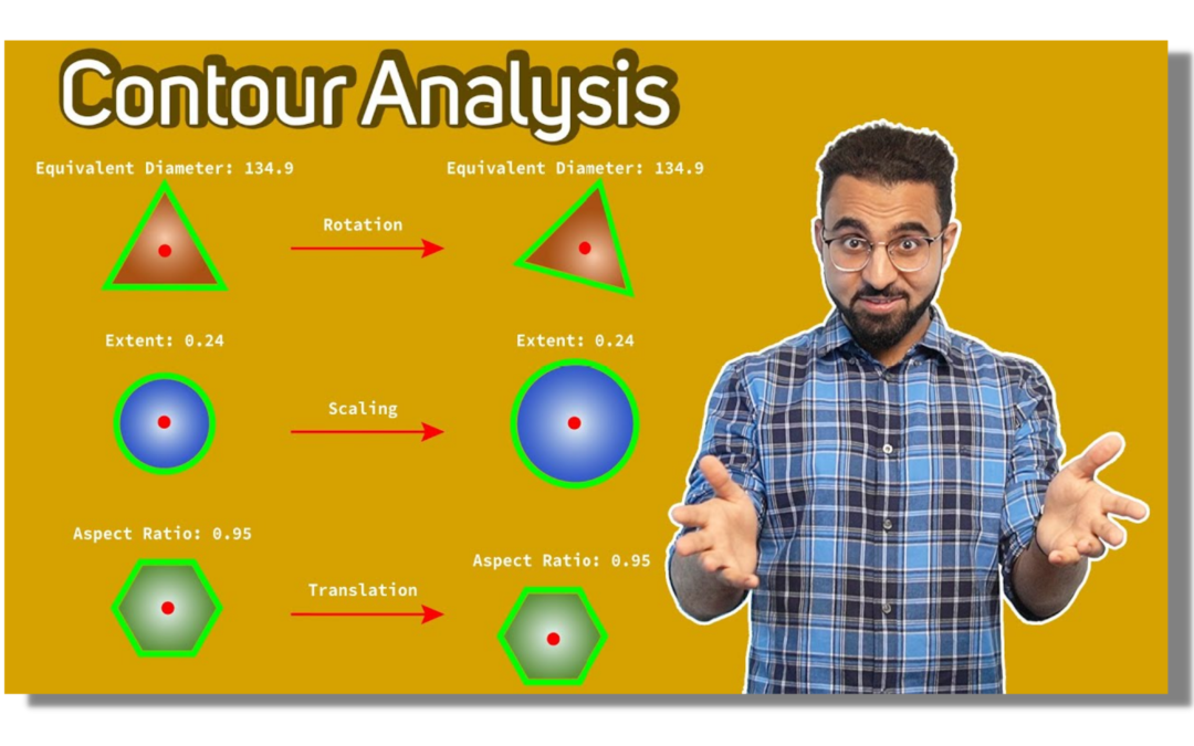
So far in our Contour Detection 101 series, we have made significant progress unpacking many of the techniques and tools that you will need to build useful vision applications. In part 1, we learned the basics, how to detect and draw the contours, in part 2 we learned to do some contour manipulations.
Now in the third part of this series, we will be learning about analyzing contours. This is really important because by doing contour analysis you can actually recognize the object being detected and differentiate one contour from another. We will also explore how you can identify different properties of contours to retrieve useful information. Once you start analyzing the contours, you can do all sorts of cool things with them. The application below that I made, uses contour analysis to detect the shapes being drawn!
So if you haven’t seen any of the previous posts make sure you do check them out since in this part we are going to build upon what we have learned before so it will be helpful to have the basics straightened out if you are new to contour detection.
Alright, now we can get started with the Code.
Download Code
[optin-monster slug=”lrrdqnjzfuycvuetarn2″]
Import the Libraries
Let’s start by importing the required libraries.
import cv2
import math
import numpy as np
import pandas as pd
import transformations
import matplotlib.pyplot as plt
Read an Image
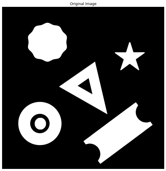
Next, let’s read an image containing a bunch of shapes.
# Read the image
image1 = cv2.imread('media/image.png')

# Display the image
plt.figure(figsize=[10,10])
plt.imshow(image1[:,:,::-1]);plt.title("Original Image");plt.axis("off");
Detect and draw Contours
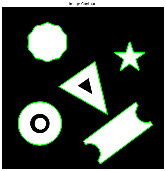
Next, we will detect and draw external contours on the image usingcv2.findContours() and cv2.drawContours() functions that we have also discussed thoroughly in the previous posts.
image1_copy = image1.copy()

# Convert to grayscale
gray_scale = cv2.cvtColor(image1_copy,cv2.COLOR_BGR2GRAY)

# Find all contours in the image
contours, hierarchy = cv2.findContours(gray_scale, cv2.RETR_EXTERNAL, cv2.CHAIN_APPROX_NONE)

# Draw all the contours.
contour_image = cv2.drawContours(image1_copy, contours, -1, (0,255,0), 3);

# Display the results.
plt.figure(figsize=[10,10])
plt.imshow(contour_image[:,:,::-1]);plt.title("Image Contours");plt.axis("off");
The result is a list of detected contours that can now be further analyzed for their properties. These properties are going to prove to be really useful when we build a vision application using contours. We will use them to provide us with valuable information about an object in the image and distinguish it from the other objects.
Below we will look at how you can retrieve some of these properties.
Image Moments
Image moments are like the weighted average of the pixel intensities in the image. They help calculate some features like the center of mass of the object, area of the object, etc. Finding image moments is a simple process in OpenCV which we can get by using the function cv2.moments() that returns a dictionary of various properties to use.
The values returned represent different kinds of image movements including raw moments, central moments, scale/rotation invariant moments, and so on.
For more information on image moments and how they are calculated, you can read this Wikipedia article. Below we will discuss how some of the image moments can be used to analyze the contours detected.
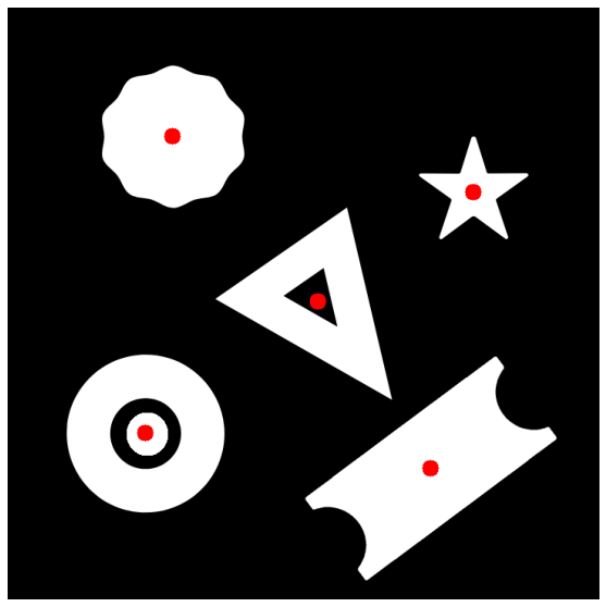
Find the center of a contour
Let’s start by finding the centroid of the object in the image using the contour’s image moments. The X and Y coordinates of the Centroid are given by two relations of the central image moments, Cx=M10/M00 and Cy=M01/M00.
# Calculate the X-coordinate of the centroid
cx = int(M['m10'] / M['m00'])

# Calculate the Y-coordinate of the centroid
cy = int(M['m01'] / M['m00'])

# Print the centroid point
print('Centroid: ({},{})'.format(cx,cy))
Centroid: (167,517)
Let’s repeat the process for the rest of the contours detected and draw a circle using cv2.circle() to indicate the centroids on the image.
image1_copy = image1.copy()

# Loop over the contours
for contour in contours:

    # Get the image moments for the contour
    M = cv2.moments(contour)

    # Calculate the centroid
    cx = int(M['m10'] / M['m00'])
    cy = int(M['m01'] / M['m00'])

    # Draw a circle to indicate the contour
    cv2.circle(image1_copy,(cx,cy), 10, (0,0,255), -1)

# Display the results
plt.figure(figsize=[10,10])
plt.imshow(image1_copy[:,:,::-1]);plt.axis("off");
Finding Contour Area
We are already familiar with one way of finding the area of contour in the last post, using function cv2.contourArea().
# Select a contour
contour = contours[1]

# Get the area of the selected contour
area_method1 = cv2.contourArea(contour)

print('Area:',area_method1)
Area: 28977.5
Additionally, you can also find the area using the m00 moment of the contour which contains the contour’s area.
# get selected contour moments
M = cv2.moments(contour)

# Get the moment containing the Area
area_method2 = M['m00']

print('Area:',area_method2)
Area: 28977.5
As you can see, both of the methods give the same result.
Contour Properties
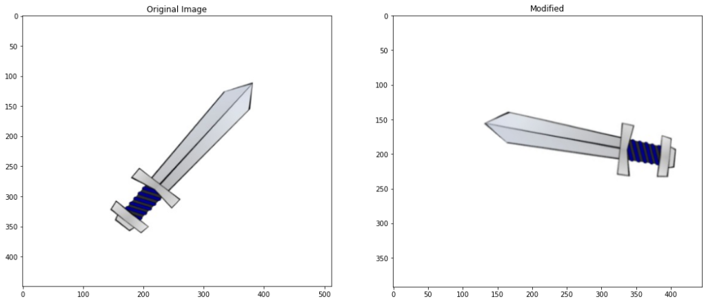
When building an application using contours, information about the properties of a contour is vital. These properties are often invariant to one or more transformations such as translation, scaling, and rotation. Below, we will have a look at some of these properties.
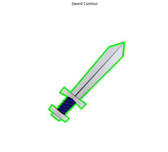
Let’s start by detecting the external contours of an image.
# Read the image
image4 = cv2.imread('media/sword.jpg')

# Create a copy
image4_copy = image4.copy()

# Convert to gray-scale
imageGray = cv2.cvtColor(image4_copy,cv2.COLOR_BGR2GRAY)

# create a binary thresholded image
_, binary = cv2.threshold(imageGray, 220, 255, cv2.THRESH_BINARY_INV)

# Detect and draw external contour
contours, hierarchy = cv2.findContours(binary, cv2.RETR_EXTERNAL, cv2.CHAIN_APPROX_NONE)

# Select a contour
contour = contours[0]

# Draw the selected contour
cv2.drawContours(image4_copy, contour, -1, (0,255,0), 3)

# Display the result
plt.figure(figsize=[10,10])
plt.imshow(image4_copy[:,:,::-1]);plt.title("Sword Contour");plt.axis("off");
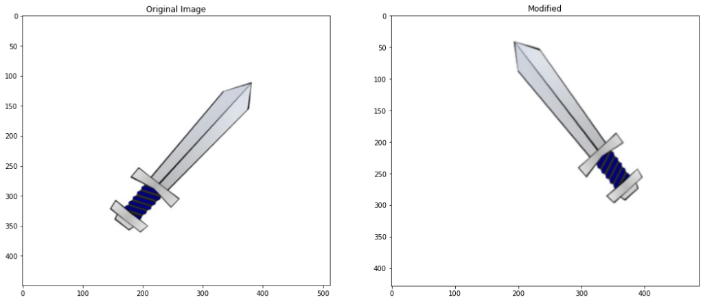
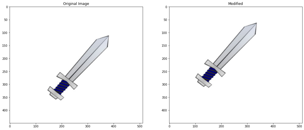
Now using a custom transform() function from the transformation.py module which you will find included with the code for this post, we can conveniently apply and display different transformations to an image.
Applied Translation of x: 44, y: 30 Applied rotation of angle: 80 Image resized to: 95.0
Aspect ratio
Aspect ratio is the ratio of width to height of the bounding rectangle of an object. It can be calculated as AR=width/height. This value is always invariant to translation.
# Get the up-right bounding rectangle for the image
x,y,w,h = cv2.boundingRect(contour)

# calculate the aspect ratio
aspect_ratio = float(w)/h
print("Aspect ratio intitially {}".format(aspect_ratio))

# Apply translation to the image and get its detected contour
modified_contour = transformations.transform(translate=True)

# Get the bounding rectangle for the detected contour
x,y,w,h = cv2.boundingRect(modified_contour)

# Calculate the aspect ratio for the modified contour
aspect_ratio = float(w)/h
print("Aspect ratio After Modification {}".format(aspect_ratio))
Aspect ratio initially 0.9442231075697212 Applied Translation of x: -45 , y: -49 Aspect ratio After Modification 0.9442231075697212
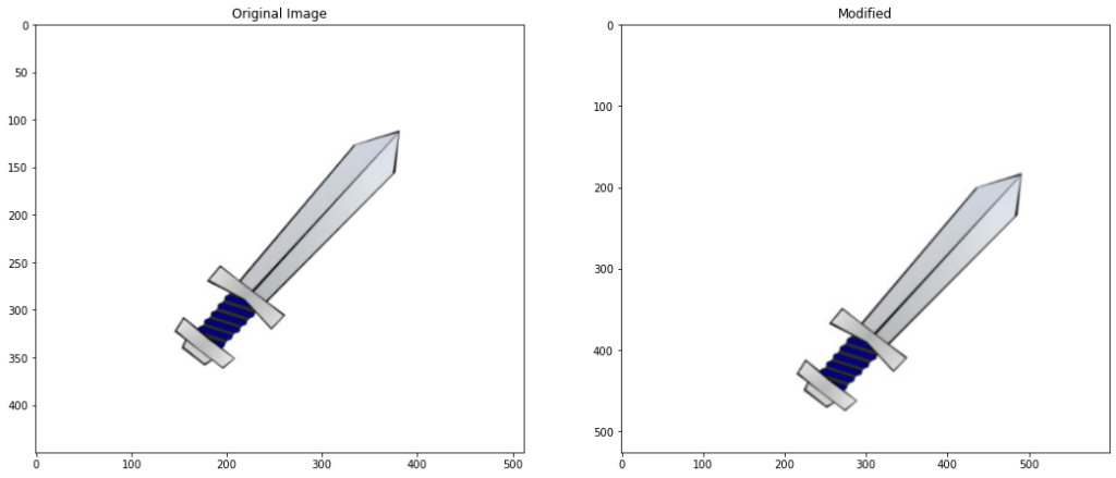
Extent
Another useful property is the extent of a contour which is the ratio of contour area to its bounding rectangle area. Extent is invariant to Translation & Scaling.
To find the extend we start by calculating the contour area for the selected contour using the function cv2.contourArea(). Next, the bounding rectangle is found using cv2.boundingRect(). The area of the bounding rectangle is calculated using rectarea=width×height. Finally, the extent is then calculated as extent=contourarea/rectarea.
# Calculate the area for the contour
original_area = cv2.contourArea(contour)

# find the bounding rectangle for the contour
x,y,w,h = cv2.boundingRect(contour)

# calculate the area for the bounding rectangle
rect_area = w*h

# calcuate the extent
extent = float(original_area)/rect_area
print("Extent intitially {}".format(extent))

# apply scaling and translation to the image and get the contour
modified_contour = transformations.transform(translate=True,scale = True)

# Get the area of modified contour
modified_area = cv2.contourArea(modified_contour)

# Get the bounding rectangle
x,y,w,h = cv2.boundingRect(modified_contour)

# Calculate the area for the bounding rectangle
modified_rect_area = w*h

# calcuate the extent
extent = float(modified_area)/modified_rect_area

print("Extent After Modification {}".format(extent))
Extent intitially 0.2404054667406324 Applied Translation of x: 38 , y: 44 Image resized to: 117.0% Extent After Modification 0.24218788234718347
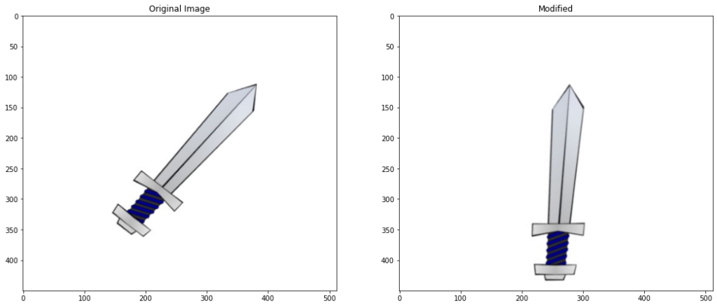
Equivalent Diameter
Equivalent Diameter is the diameter of the circle whose area is the same as the contour area. It is Invariant to Translation & Rotation. The equivalent diameter can be calculated by first getting the area of contour with cv2.boundingRect(), the area of the circle is given by area=2×π×d2/4 where d is the diameter of the circle.
So to find the diameter we just have to make d the subject in the above equation, giving us: d= √(4×rectArea/π).
# Calculate the diameter
equi_diameter = np.sqrt(4*original_area/np.pi)
print("Equi diameter intitially {}".format(equi_diameter))

# Apply rotation and transformation
modified_contour = transformations.transform(rotate= True)

# Get the area of modified contour
modified_area = cv2.contourArea(modified_contour)

# Calculate the diameter
equi_diameter = np.sqrt(4*modified_area/np.pi)
print("Equi diameter After Modification {}".format(equi_diameter))
Equi diameter intitially 134.93924087995146 Applied Translation of x: -39 , y: 38 Applied rotation of angle: 38 Equi diameter After Modification 135.06184863765444
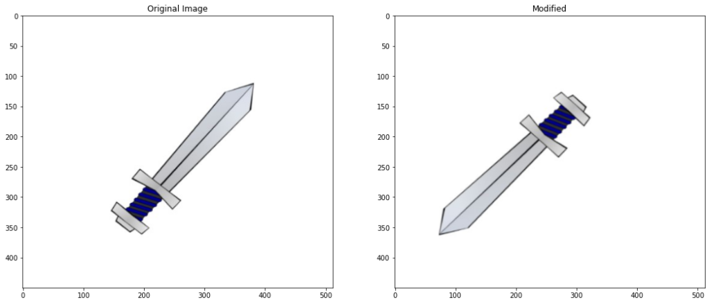
Orientation
Orientation is simply the angle at which an object is rotated.
# Rotate and translate the contour
modified_contour = transformations.transform(translate=True,rotate= True,display = True)
Applied Translation of x: 48 , y: -37 Applied rotation of angle: 176
Now Let’s take a look at an elliptical angle on the sword contour above
# Fit and ellipse onto the contour similarly to minimum area rectangle
(x,y),(MA,ma),angle = cv2.fitEllipse(modified_contour)

# Print the angle of rotation of ellipse
print("Elliptical Angle is {}".format(angle))
Elliptical Angle is 46.882904052734375
Below method also gives the angle of the contour by fitting a rotated box instead of an ellipse
(x,y),(w,mh),angle = cv2.minAreaRect(modified_contour)
print("RotatedRect Angle is {}".format(angle))
RotatedRect Angle is 45.0
Note:Don’t be confused by why all three angles are showing different results, they all calculate angles differently, for e.g ellipse fits an ellipse and then calculates the angle that an ellipse makes, similarly the rotated rectangle calculates the angle the rectangle makes. For triggering decisions based on the calculated angle you would first need to find what angle the respective method is making at the given orientations of the object.
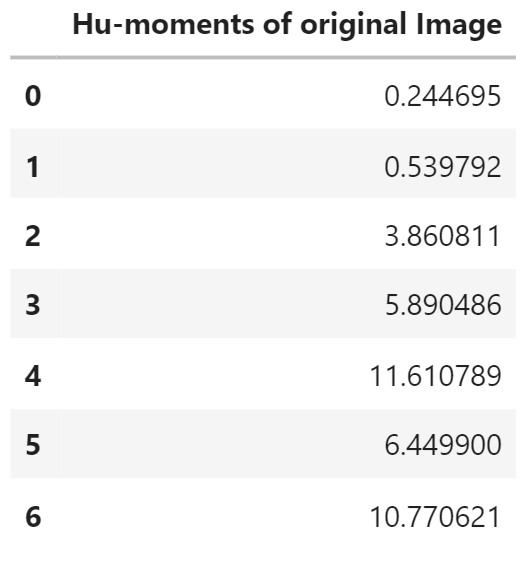
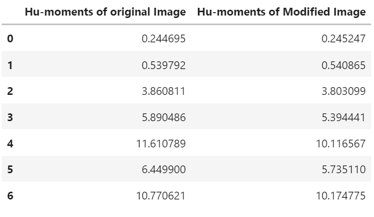
Hu moments
Hu moments are a set of 7 numbers calculated using the central moments. What makes these 7 moments special is the fact that out of these 7 moments, the first 6 of the Hu moments are invariant to translation, scaling, rotation and reflection. The 7th Hu moment is also invariant to these transformations, except that it changes its sign in case of reflection. Below we will calculate the Hu moments for the sword contour, using the moments of the contour.
You can read this paper if you want to know more about hu-moments and how they are calculated.
# Calculate moments
M = cv2.moments(contour)

# Calculate Hu Moments
hu_M = cv2.HuMoments(M)

print(hu_M)
As you can see the different hu-moments have varying ranges (e.g. compare hu-moment 1 and 7) so to make the Hu-moments more comparable with each other, we will transform them to log-scale and bring them all to the same range.
# Log scale hu moments
for i in range(0,7):
    hu_M[i] = -1* math.copysign(1.0,  hu_M[i]) * math.log10(abs(hu_M[i]))

df = pd.DataFrame(hu_M,columns=['Hu-moments of original Image'])
df
Next up let’s apply transformations to the image and find the Hu-moments again.
# Apply translation to the image and get its detected contour
modified_contour = transformations.transform(translate = True, scale = True, rotate = True)
Applied Translation of x: -31 , y: 48 Applied rotation of angle: 122 Image resized to: 87.0%
# Calculate moments
M_modified = cv2.moments(modified_contour)

# Calculate Hu Moments
hu_Modified = cv2.HuMoments(M_modified)

# Log scale hu moments
for i in range(0,7):
    hu_Modified[i] = -1* math.copysign(1.0, hu_Modified[i]) * math.log10(abs(hu_Modified[i]))

df['Hu-moments of Modified Image'] = hu_Modified
df
The difference is minimal because of the invariance of Hu-moments to the applied transformations.
[optin-monster slug=”d8wgq6fdm5mppdb5fi99″]
Summary
In this post, we saw how useful contour detection can be when you analyze the detected contour for its properties, enabling you to build applications capable of detecting and identifying objects in an image.
We learned how image moments can provide us useful information about a contour such as the center of a contour or the area of contour.
We also learned how to calculate different contour properties invariant to different transformations such as rotation, translation, and scaling.
Lastly, we also explored seven unique image moments called Hu-moments which are really helpful for object detection using contours since they are invariant to translation, scaling, rotation, and reflection at once.
This concludes the third part of the series. In the next and final part of the series, we will be building a Vehicle Detection Application using many of the techniques we have learned in this series.
You can reach out to me personally for a 1 on 1 consultation session in AI/computer vision regarding your project. Our talented team of vision engineers will help you every step of the way. Get on a call with me directlyhere.
Ready to seriously dive into State of the Art AI & Computer Vision? Then Sign up for these premium Courses by Bleed AI
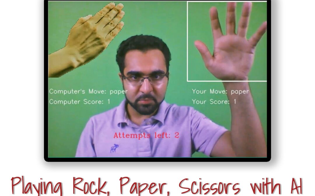
You think of your move and I’ll make mine below this line in 1…2…and 3.
I choose ROCK.
Well? …who won. It doesn’t matter cause you probably glanced at the word “ROCK” before thinking about a move or maybe you didn’t pay any heed to my feeble attempt at playing rock, paper, scissor with you in a blog post.
So why am I making some miserable attempts trying to play this game in text with you?
Let’s just say, a couple of months down the road in lockdown you just run out of fun ideas. To be honest I desperately need to socialize and do something fun.
Ideally, I would love to play games with some good friends, …or just friends…or anyone who is willing to play.
Now I’m tired of video games. I want to go for something old fashioned, like something involving other intelligent beings, ideally a human. But because of the lockdown, we’re a bit short on those for close proximity activities. So what’s the next best thing?
AI of course. So yeah why not build an AI that would play with me whenever I want.
Now I don’t want to make a dumb AI bot that predicts randomly between rock, paper, and scissor, but rather I also don’t want to use any keyboard inputs or mouse. Just want to play the old fashioned way.
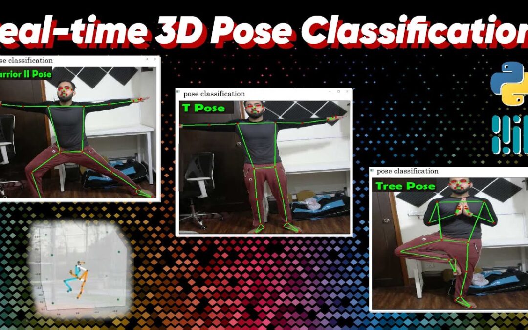
In this tutorial, we’ll learn how to do real-time 3D pose detection using the mediapipe library in python. After that, we’ll calculate angles between body joints and combine them with some heuristics to create a pose classification system.
All of this will work on real-time camera feed using your CPU as well as on images. See results below.
The code is really simple, for detailed code explanation do also check out the YouTube tutorial, although this blog post will suffice enough to get the code up and running in no time.
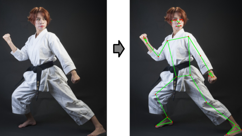
Pose Detection or Pose Estimation is a very popular problem in computer vision, in fact, it belongs to a broader class of computer vision domain called key point estimation. Today we’ll learn to do Pose Detection where we’ll try to localize 33 key body landmarks on a person e.g. elbows, knees, ankles, etc. see the image below:
Some interesting applications of pose detection are:
Full body Gesture Control to control anything from video games (e.g. kinect) to physical appliances, robots etc. Check this.
Creating Augmented reality applications that overlay virtual clothes or other accessories over someone’s body. Check this.
Now, these are just some interesting things you can make using pose detection, as you can see it’s a really interesting problem.
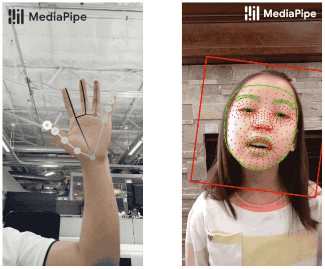
And that’s not it there are other types of key point detection problems too, e.g. facial landmark detection, hand landmark detection, etc.
We will actually learn to do both of the above in the upcoming tutorials.
Key point detection in turn belongs to a major computer vision branch called Image recognition, other broad classes of vision that belong in this branch are Classification, Detection, and Segmentation.
Here’s a very generic definition of each class.
In classificationwe try to classify whole images or videos as belonging to a certain class.
In Detection we try to classify and localize objects or classes of interest.
In Segmentation, we try to extract/segment or find the exact boundary/outline of our target object/class.
In Keypoint Detection, we try to localize predefined points/landmarks.
If you’re new to Computer vision and just exploring the waters, check this page from paperswithcode, it lists a lot of subcategories from the above major categories. Now don’t be confused by the categorization that paperswtihcode has done, personally speaking, I don’t agree with the way they have sorted subcategories with applications and there are some other issues. The takeaway is that there are a lot of variations in computer vision problems, but the 4 categories I’ve listed above are some major ones.
Part 1 (b): Mediapipe’s Pose Detection Implementation:
Here’s a brief introduction to Mediapipe;
“Mediapipe is a cross-platform/open-source tool that allows you to run a variety of machine learning models in real-time. It’s designed primarily for facilitating the use of ML in streaming media & It was built by Google”
Not only is this tool backed by google but models in Mediapipe are actively used in Google products. So you can expect nothing less than the state of the Art performance from this library.
Now MediaPipe’s Pose detection is a State of the Art solution for high-fidelity (i.e. high quality) and low latency (i.e. Damn fast) for detecting 33 3D landmarks on a person in real-time video feeds on low-end devices i.e. phones, laptops, etc.
Alright, so what makes this pose detection model from Mediapipe so fast?
They are actually using a very successful deep learning recipe that is creating a 2 step detector, where you combine a computationally expensive object detector with a lightweight object tracker.
Here’s how this works:
You run the detector in the first frame of the video to localize the person and provide a bounding box around it, after that the tracker takes over and it predicts the landmark points inside that bounding box ROI, the tracker continues to run on any subsequent frames in the video using the previous frame’s ROI and only calls the detection model again when it fails to track the person with high confidence.
Their model works best if the person is standing 2-4 meters away from the camera and one major limitation of their model is that this approach only works for single-person pose detection, it’s not applicable for multi-person detection.
Mediapipe actually trained 3 models, with different tradeoffs between speed and performance. You’ll be able to use all 3 of them with mediapipe.
The detector used in pose detection is inspired by Mediapiep’s lightweight BlazeFace model, you can read this paper. For the landmark model used in pose detection, you can read this paper for more details.or readGoogle’s blogon it.
Here are the 33 landmarks that this model detects:
Alright now that we have covered some basic theory and implementation details, let’s get into the code.
Download Code
[optin-monster slug=”kalfyxphljhqu1zouums”]
Part 2: Using Pose Detection in images and on videos
Import the Libraries
Let’s start by importing the required libraries.
import math
import cv2
import numpy as np
from time import time
import mediapipe as mp
import matplotlib.pyplot as plt
Initialize the Pose Detection Model
The first thing that we need to do is initialize the pose class using the mp.solutions.pose syntax and then we will call the setup function mp.solutions.pose.Pose() with the arguments:
static_image_mode – It is a boolean value that is if set to False, the detector is only invoked as needed, that is in the very first frame or when the tracker loses track. If set to True, the person detector is invoked on every input image. So you should probably set this value to True when working with a bunch of unrelated images not videos. Its default value is False.
min_detection_confidence – It is the minimum detection confidence with range (0.0 , 1.0) required to consider the person-detection model’s prediction correct. Its default value is 0.5. This means if the detector has a prediction confidence of greater or equal to 50% then it will be considered as a positive detection.
min_tracking_confidence – It is the minimum tracking confidence ([0.0, 1.0]) required to consider the landmark-tracking model’s tracked pose landmarks valid. If the confidence is less than the set value then the detector is invoked again in the next frame/image, so increasing its value increases the robustness, but also increases the latency. Its default value is 0.5.
model_complexity – It is the complexity of the pose landmark model. As there are three different models to choose from so the possible values are 0, 1, or 2. The higher the value, the more accurate the results are, but at the expense of higher latency. Its default value is 1.
smooth_landmarks – It is a boolean value that is if set to True, pose landmarks across different frames are filtered to reduce noise. But only works when static_image_mode is also set to False. Its default value is True.
Then we will also initialize mp.solutions.drawing_utils class that will allow us to visualize the landmarks after detection, instead of using this, you can also use OpenCV to visualize the landmarks.
# Initializing mediapipe pose class.
mp_pose = mp.solutions.pose

# Setting up the Pose function.
pose = mp_pose.Pose(static_image_mode=True, min_detection_confidence=0.3, model_complexity=2)

# Initializing mediapipe drawing class, useful for annotation.
mp_drawing = mp.solutions.drawing_utils
Downloading model to C:\ProgramData\Anaconda3\lib\site-packages\mediapipe/modules/pose_landmark/pose_landmark_heavy.tflite
Read an Image
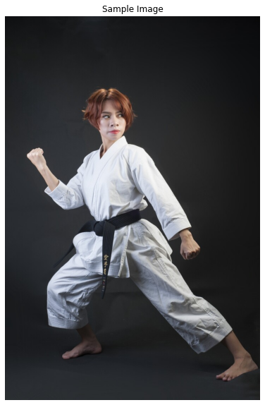
Now we will read a sample image using the function cv2.imread() and then display that image using the matplotlib library.
# Read an image from the specified path.
sample_img = cv2.imread('media/sample.jpg')

# Specify a size of the figure.
plt.figure(figsize = [10, 10])

# Display the sample image, also convert BGR to RGB for display.
plt.title("Sample Image");plt.axis('off');plt.imshow(sample_img[:,:,::-1]);plt.show()
Perform Pose Detection
Now we will pass the image to the pose detection machine learning pipeline by using the function mp.solutions.pose.Pose().process(). But the pipeline expects the input images in RGB color format so first we will have to convert the sample image from BGR to RGB format using the function cv2.cvtColor() as OpenCV reads images in BGR format (instead of RGB).
After performing the pose detection, we will get a list of thirty-three landmarks representing the body joint locations of the prominent person in the image. Each landmark has:
x – It is the landmark x-coordinate normalized to [0.0, 1.0] by the image width.
y: It is the landmark y-coordinate normalized to [0.0, 1.0] by the image height.
z: It is the landmark z-coordinate normalized to roughly the same scale as x. It represents the landmark depth with midpoint of hips being the origin, so the smaller the value of z, the closer the landmark is to the camera.
visibility: It is a value with range [0.0, 1.0] representing the possibility of the landmark being visible (not occluded) in the image. This is a useful variable when deciding if you want to show a particular joint because it might be occluded or partially visible in the image.
After performing the pose detection on the sample image above, we will display the first two landmarks from the list, so that you get a better idea of the output of the model.
# Perform pose detection after converting the image into RGB format.
results = pose.process(cv2.cvtColor(sample_img, cv2.COLOR_BGR2RGB))

# Check if any landmarks are found.
if results.pose_landmarks:

    # Iterate two times as we only want to display first two landmarks.
    for i in range(2):

        # Display the found normalized landmarks.
        print(f'{mp_pose.PoseLandmark(i).name}:\n{results.pose_landmarks.landmark[mp_pose.PoseLandmark(i).value]}')
Now we will convert the two normalized landmarks displayed above into their original scale by using the width and height of the image.
# Retrieve the height and width of the sample image.
image_height, image_width, _ = sample_img.shape

# Check if any landmarks are found.
if results.pose_landmarks:

    # Iterate two times as we only want to display first two landmark.
    for i in range(2):

        # Display the found landmarks after converting them into their original scale.
        print(f'{mp_pose.PoseLandmark(i).name}:')
        print(f'x: {results.pose_landmarks.landmark[mp_pose.PoseLandmark(i).value].x * image_width}')
        print(f'y: {results.pose_landmarks.landmark[mp_pose.PoseLandmark(i).value].y * image_height}')
        print(f'z: {results.pose_landmarks.landmark[mp_pose.PoseLandmark(i).value].z * image_width}')
        print(f'visibility: {results.pose_landmarks.landmark[mp_pose.PoseLandmark(i).value].visibility}\n')
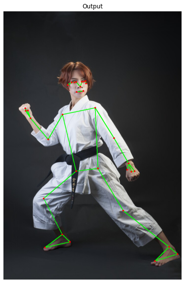
Now we will draw the detected landmarks on the sample image using the function mp.solutions.drawing_utils.draw_landmarks() and display the resultant image using the matplotlib library.
# Create a copy of the sample image to draw landmarks on.
img_copy = sample_img.copy()

# Check if any landmarks are found.
if results.pose_landmarks:

    # Draw Pose landmarks on the sample image.
    mp_drawing.draw_landmarks(image=img_copy, landmark_list=results.pose_landmarks, connections=mp_pose.POSE_CONNECTIONS)

    # Specify a size of the figure.
    fig = plt.figure(figsize = [10, 10])

    # Display the output image with the landmarks drawn, also convert BGR to RGB for display.
    plt.title("Output");plt.axis('off');plt.imshow(img_copy[:,:,::-1]);plt.show()
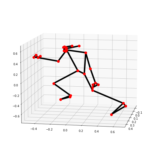
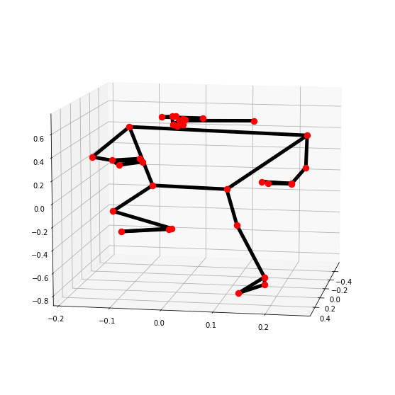
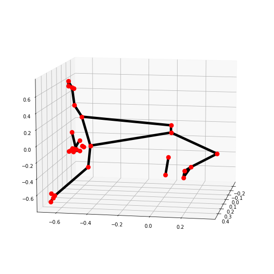
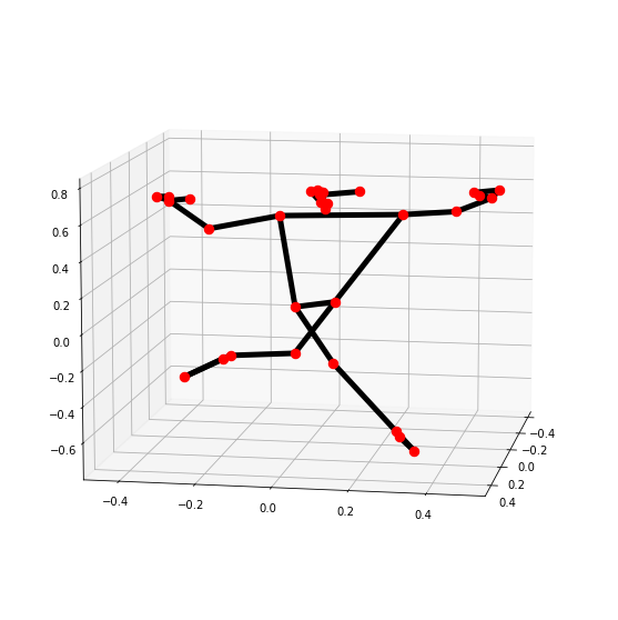
Now we will go a step further and visualize the landmarks in three-dimensions (3D) using the function mp.solutions.drawing_utils.plot_landmarks(). We will need the POSE_WORLD_LANDMARKS that is another list of pose landmarks in world coordinates that has the 3D coordinates in meters with the origin at the center between the hips of the person.
# Plot Pose landmarks in 3D.
mp_drawing.plot_landmarks(results.pose_world_landmarks, mp_pose.POSE_CONNECTIONS)
Note: This is actually a neat hack by mediapipe, the coordinates returned are not actually in 3D but by setting hip landmark as the origin allows us to measure the relative distance of the other points from the hip, and since this distance increases or decreases depending upon if you’re close or further from the camera it gives us a sense of the depth of each landmark point.
Create a Pose Detection Function
Now we will put all this together to create a function that will perform pose detection on an image and visualize the results or return the results depending upon the passed arguments.
def detectPose(image, pose, display=True):
'''
This function performs pose detection on an image.
Args:
image: The input image with a prominent person whose pose landmarks needs to be detected.
pose: The pose setup function required to perform the pose detection.
display: A boolean value that is if set to true the function displays the original input image, the resultant image,
and the pose landmarks in 3D plot and returns nothing.
Returns:
output_image: The input image with the detected pose landmarks drawn.
landmarks: A list of detected landmarks converted into their original scale.
'''
# Create a copy of the input image.
output_image = image.copy()
# Convert the image from BGR into RGB format.
imageRGB = cv2.cvtColor(image, cv2.COLOR_BGR2RGB)
# Perform the Pose Detection.
results = pose.process(imageRGB)
# Retrieve the height and width of the input image.
height, width, _ = image.shape
# Initialize a list to store the detected landmarks.
landmarks = []
# Check if any landmarks are detected.
if results.pose_landmarks:
# Draw Pose landmarks on the output image.
mp_drawing.draw_landmarks(image=output_image, landmark_list=results.pose_landmarks,
connections=mp_pose.POSE_CONNECTIONS)
# Iterate over the detected landmarks.
for landmark in results.pose_landmarks.landmark:
# Append the landmark into the list.
landmarks.append((int(landmark.x * width), int(landmark.y * height),
(landmark.z * width)))
# Check if the original input image and the resultant image are specified to be displayed.
if display:
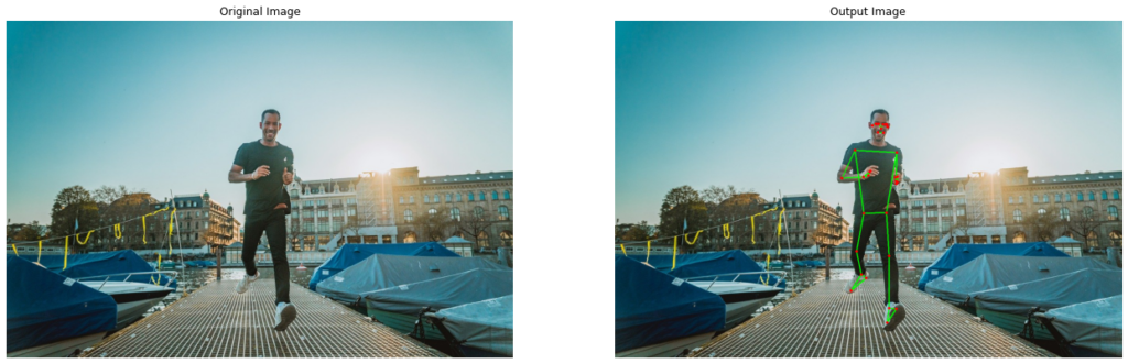
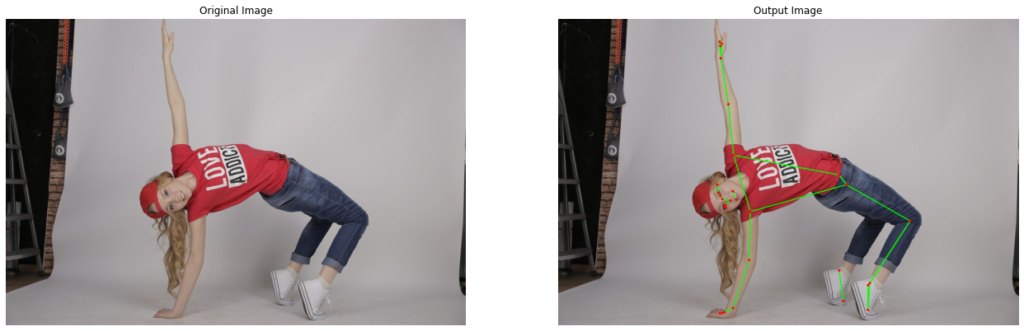
# Display the original input image and the resultant image.
plt.figure(figsize=[22,22])
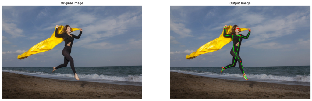
plt.subplot(121);plt.imshow(image[:,:,::-1]);plt.title("Original Image");plt.axis('off');
plt.subplot(122);plt.imshow(output_image[:,:,::-1]);plt.title("Output Image");plt.axis('off');
# Also Plot the Pose landmarks in 3D.
mp_drawing.plot_landmarks(results.pose_world_landmarks, mp_pose.POSE_CONNECTIONS)
# Otherwise
else:
# Return the output image and the found landmarks.
return output_image, landmarks
Now we will utilize the function created above to perform pose detection on a few sample images and display the results.
# Read another sample image and perform pose detection on it.
image = cv2.imread('media/sample1.jpg')
detectPose(image, pose, display=True)
# Read another sample image and perform pose detection on it.
image = cv2.imread('media/sample2.jpg')
detectPose(image, pose, display=True)
# Read another sample image and perform pose detection on it.
image = cv2.imread('media/sample3.jpg')
detectPose(image, pose, display=True)
Pose Detection On Real-Time Webcam Feed/Video
The results on the images were pretty good, now we will try the function on a real-time webcam feed and a video. Depending upon whether you want to run pose detection on a video stored in the disk or on the webcam feed, you can comment and uncomment the initialization code of the VideoCapture object accordingly.
# Setup Pose function for video.
pose_video = mp_pose.Pose(static_image_mode=False, min_detection_confidence=0.5, model_complexity=1)

# Initialize the VideoCapture object to read from the webcam.
#video = cv2.VideoCapture(0)

# Initialize the VideoCapture object to read from a video stored in the disk.
video = cv2.VideoCapture('media/running.mp4')


# Initialize a variable to store the time of the previous frame.
time1 = 0

# Iterate until the video is accessed successfully.
while video.isOpened():

    # Read a frame.
    ok, frame = video.read()

    # Check if frame is not read properly.
    if not ok:

        # Break the loop.
        break

    # Flip the frame horizontally for natural (selfie-view) visualization.
    frame = cv2.flip(frame, 1)

    # Get the width and height of the frame
    frame_height, frame_width, _ =  frame.shape

    # Resize the frame while keeping the aspect ratio.
    frame = cv2.resize(frame, (int(frame_width * (640 / frame_height)), 640))

    # Perform Pose landmark detection.
    frame, _ = detectPose(frame, pose_video, display=False)

    # Set the time for this frame to the current time.
    time2 = time()

    # Check if the difference between the previous and this frame time > 0 to avoid division by zero.
    if (time2 - time1) > 0:

        # Calculate the number of frames per second.
        frames_per_second = 1.0 / (time2 - time1)

        # Write the calculated number of frames per second on the frame.
        cv2.putText(frame, 'FPS: {}'.format(int(frames_per_second)), (10, 30),cv2.FONT_HERSHEY_PLAIN, 2, (0, 255, 0), 3)

    # Update the previous frame time to this frame time.
    # As this frame will become previous frame in next iteration.
    time1 = time2

    # Display the frame.
    cv2.imshow('Pose Detection', frame)

    # Wait until a key is pressed.
    # Retreive the ASCII code of the key pressed
    k = cv2.waitKey(1) & 0xFF

    # Check if 'ESC' is pressed.
    if(k == 27):

        # Break the loop.
        break

# Release the VideoCapture object.
video.release()

# Close the windows.
cv2.destroyAllWindows()
Output:
Cool! so it works great on the videos too. The model is pretty fast and accurate.
Part 3: Pose Classification with Angle Heuristics
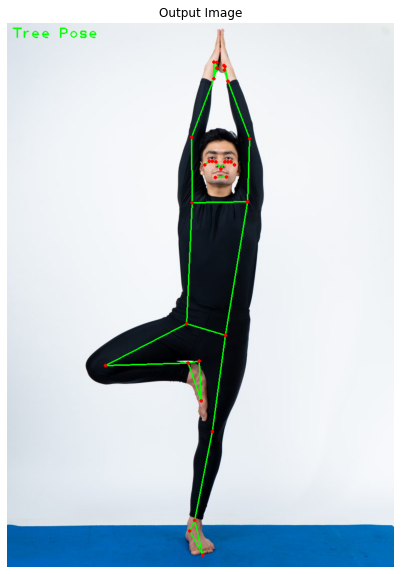
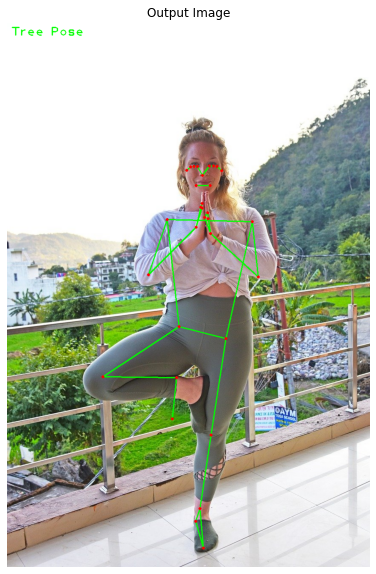
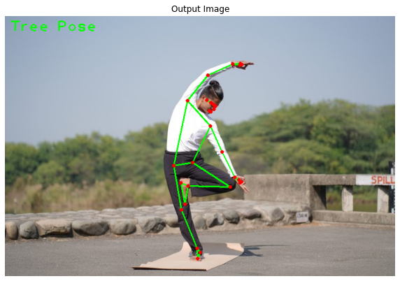
We have learned to perform pose detection, now we will level up our game by also classifying different yoga poses using the calculated angles of various joints. We will first detect the pose landmarks and then use them to compute angles between joints and depending upon those angles we will recognize the yoga pose of the prominent person in an image.
But this approach does have a drawback that limits its use to a controlled environment, the calculated angles vary with the angle between the person and the camera. So the person needs to be facing the camera straight to get the best results.
Create a Function to Calculate Angle between Landmarks
Now we will create a function that will be capable of calculating angles between three landmarks. The angle between landmarks? Do not get confused, as this is the same as calculating the angle between two lines.
The first point (landmark) is considered as the starting point of the first line, the second point (landmark) is considered as the ending point of the first line and the starting point of the second line as well, and the third point (landmark) is considered as the ending point of the second line.
def calculateAngle(landmark1, landmark2, landmark3):
    '''
    This function calculates angle between three different landmarks.
    Args:
        landmark1: The first landmark containing the x,y and z coordinates.
        landmark2: The second landmark containing the x,y and z coordinates.
        landmark3: The third landmark containing the x,y and z coordinates.
    Returns:
        angle: The calculated angle between the three landmarks.

    '''

    # Get the required landmarks coordinates.
    x1, y1, _ = landmark1
    x2, y2, _ = landmark2
    x3, y3, _ = landmark3

    # Calculate the angle between the three points
    angle = math.degrees(math.atan2(y3 - y2, x3 - x2) - math.atan2(y1 - y2, x1 - x2))

    # Check if the angle is less than zero.
    if angle < 0:

        # Add 360 to the found angle.
        angle += 360

    # Return the calculated angle.
    return angle
Now we will test the function created above to calculate angle three landmarks with dummy values.
# Calculate the angle between the three landmarks.
angle = calculateAngle((558, 326, 0), (642, 333, 0), (718, 321, 0))

# Display the calculated angle.
print(f'The calculated angle is {angle}')
The calculated angle is 166.26373169437744
Create a Function to Perform Pose Classification
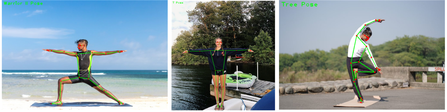
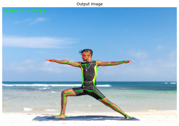
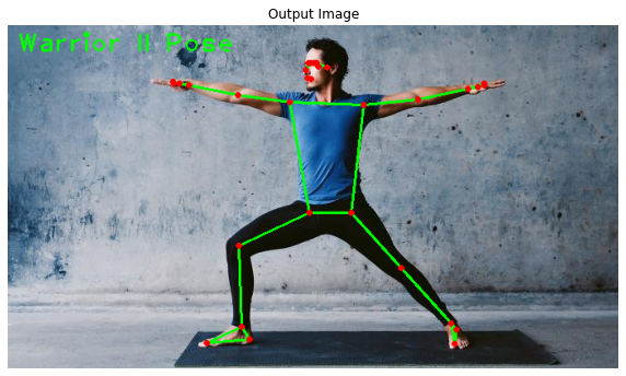
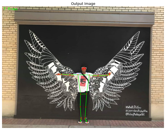
Now we will create a function that will be capable of classifying different yoga poses using the calculated angles of various joints. The function will be capable of identifying the following yoga poses:
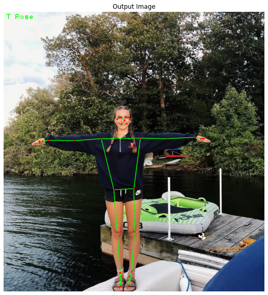
Warrior II Pose
T Pose
Tree Pose
def classifyPose(landmarks, output_image, display=False):
'''
This function classifies yoga poses depending upon the angles of various body joints.
Args:
landmarks: A list of detected landmarks of the person whose pose needs to be classified.
output_image: A image of the person with the detected pose landmarks drawn.
display: A boolean value that is if set to true the function displays the resultant image with the pose label
written on it and returns nothing.
Returns:
output_image: The image with the detected pose landmarks drawn and pose label written.
label: The classified pose label of the person in the output_image.
'''
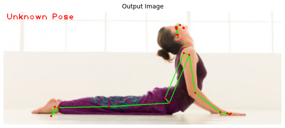
# Initialize the label of the pose. It is not known at this stage.
label = 'Unknown Pose'
# Specify the color (Red) with which the label will be written on the image.
color = (0, 0, 255)
# Calculate the required angles.
#----------------------------------------------------------------------------------------------------------------
# Get the angle between the left shoulder, elbow and wrist points.
left_elbow_angle = calculateAngle(landmarks[mp_pose.PoseLandmark.LEFT_SHOULDER.value],
landmarks[mp_pose.PoseLandmark.LEFT_ELBOW.value],
landmarks[mp_pose.PoseLandmark.LEFT_WRIST.value])
# Get the angle between the right shoulder, elbow and wrist points.
right_elbow_angle = calculateAngle(landmarks[mp_pose.PoseLandmark.RIGHT_SHOULDER.value],
landmarks[mp_pose.PoseLandmark.RIGHT_ELBOW.value],
landmarks[mp_pose.PoseLandmark.RIGHT_WRIST.value])
# Get the angle between the left elbow, shoulder and hip points.
left_shoulder_angle = calculateAngle(landmarks[mp_pose.PoseLandmark.LEFT_ELBOW.value],
landmarks[mp_pose.PoseLandmark.LEFT_SHOULDER.value],
landmarks[mp_pose.PoseLandmark.LEFT_HIP.value])
# Get the angle between the right hip, shoulder and elbow points.
right_shoulder_angle = calculateAngle(landmarks[mp_pose.PoseLandmark.RIGHT_HIP.value],
landmarks[mp_pose.PoseLandmark.RIGHT_SHOULDER.value],
landmarks[mp_pose.PoseLandmark.RIGHT_ELBOW.value])
# Get the angle between the left hip, knee and ankle points.
left_knee_angle = calculateAngle(landmarks[mp_pose.PoseLandmark.LEFT_HIP.value],
landmarks[mp_pose.PoseLandmark.LEFT_KNEE.value],
landmarks[mp_pose.PoseLandmark.LEFT_ANKLE.value])
# Get the angle between the right hip, knee and ankle points
right_knee_angle = calculateAngle(landmarks[mp_pose.PoseLandmark.RIGHT_HIP.value],
landmarks[mp_pose.PoseLandmark.RIGHT_KNEE.value],
landmarks[mp_pose.PoseLandmark.RIGHT_ANKLE.value])
#----------------------------------------------------------------------------------------------------------------
# Check if it is the warrior II pose or the T pose.
# As for both of them, both arms should be straight and shoulders should be at the specific angle.
#----------------------------------------------------------------------------------------------------------------
# Check if the both arms are straight.
if left_elbow_angle > 165 and left_elbow_angle < 195 and right_elbow_angle > 165 and right_elbow_angle < 195:
# Check if shoulders are at the required angle.
if left_shoulder_angle > 80 and left_shoulder_angle < 110 and right_shoulder_angle > 80 and right_shoulder_angle < 110:
# Check if it is the warrior II pose.
#----------------------------------------------------------------------------------------------------------------
# Check if one leg is straight.
if left_knee_angle > 165 and left_knee_angle < 195 or right_knee_angle > 165 and right_knee_angle < 195:
# Check if the other leg is bended at the required angle.
if left_knee_angle > 90 and left_knee_angle < 120 or right_knee_angle > 90 and right_knee_angle < 120:
# Specify the label of the pose that is Warrior II pose.
label = 'Warrior II Pose'
#----------------------------------------------------------------------------------------------------------------
# Check if it is the T pose.
#----------------------------------------------------------------------------------------------------------------
# Check if both legs are straight
if left_knee_angle > 160 and left_knee_angle < 195 and right_knee_angle > 160 and right_knee_angle < 195:
# Specify the label of the pose that is tree pose.
label = 'T Pose'
#----------------------------------------------------------------------------------------------------------------
# Check if it is the tree pose.
#----------------------------------------------------------------------------------------------------------------
# Check if one leg is straight
if left_knee_angle > 165 and left_knee_angle < 195 or right_knee_angle > 165 and right_knee_angle < 195:
# Check if the other leg is bended at the required angle.
if left_knee_angle > 315 and left_knee_angle < 335 or right_knee_angle > 25 and right_knee_angle < 45:
# Specify the label of the pose that is tree pose.
label = 'Tree Pose'
#----------------------------------------------------------------------------------------------------------------
# Check if the pose is classified successfully
if label != 'Unknown Pose':
# Update the color (to green) with which the label will be written on the image.
color = (0, 255, 0)
# Write the label on the output image.
cv2.putText(output_image, label, (10, 30),cv2.FONT_HERSHEY_PLAIN, 2, color, 2)
# Check if the resultant image is specified to be displayed.
if display:
# Display the resultant image.
plt.figure(figsize=[10,10])
plt.imshow(output_image[:,:,::-1]);plt.title("Output Image");plt.axis('off');
else:
# Return the output image and the classified label.
return output_image, label
Now we will utilize the function created above to perform pose classification on a few images of people and display the results.
Warrior II Pose
The Warrior II Pose (also known as Virabhadrasana II) is the same pose that the person is making in the image above. It can be classified using the following combination of body part angles:
Around 180° at both elbows
Around 90° angle at both shoulders
Around 180° angle at one knee
Around 90° angle at the other knee
# Read a sample image and perform pose classification on it.
image = cv2.imread('media/warriorIIpose.jpg')
output_image, landmarks = detectPose(image, pose, display=False)
if landmarks:
    classifyPose(landmarks, output_image, display=True)
# Read another sample image and perform pose classification on it.
image = cv2.imread('media/warriorIIpose1.jpg')
output_image, landmarks = detectPose(image, pose, display=False)
if landmarks:
    classifyPose(landmarks, output_image, display=True)
Tree Pose
Tree Pose (also known as Vrikshasana) is another yoga pose for which the person has to keep one leg straight and bend the other leg at a required angle. The pose can be classified easily using the following combination of body part angles:
Around 180° angle at one knee
Around 35° (if right knee) or 335° (if left knee) angle at the other knee
Now to understand it better, you should go back to the pose classification function above to overview the classification code of this yoga pose.
We will perform pose classification on a few images of people in the tree yoga pose and display the results using the same function we had created above.
# Read a sample image and perform pose classification on it.
image = cv2.imread('media/treepose.jpg')
output_image, landmarks = detectPose(image, mp_pose.Pose(static_image_mode=True,
                                         min_detection_confidence=0.5, model_complexity=0), display=False)
if landmarks:
    classifyPose(landmarks, output_image, display=True)
# Read another sample image and perform pose classification on it.
image = cv2.imread('media/treepose1.jpg')
output_image, landmarks = detectPose(image, mp_pose.Pose(static_image_mode=True,
                                         min_detection_confidence=0.5, model_complexity=0), display=False)
if landmarks:
    classifyPose(landmarks, output_image, display=True)
# Read another sample image and perform pose classification on it.
image = cv2.imread('media/treepose2.jpg')
output_image, landmarks = detectPose(image, pose, display=False)
if landmarks:
    classifyPose(landmarks, output_image, display=True)
T Pose
T Pose (also known as a bind pose or reference pose) is the last pose we are dealing with in this lesson. To make this pose, one has to stand up like a tree with both hands wide open as branches. The following body part angles are required to make this one:
Around 180° at both elbows
Around 90° angle at both shoulders
Around 180° angle at both knees
You can now go back to go through the classification code of this T pose in the pose classification function created above.
Now, let’s test the pose classification function on a few images of the T pose.
# Read another sample image and perform pose classification on it.
image = cv2.imread('media/Tpose.jpg')
output_image, landmarks = detectPose(image, pose, display=False)
if landmarks:
    classifyPose(landmarks, output_image, display=True)
# Read another sample image and perform pose classification on it.
image = cv2.imread('media/Tpose1.jpg')
output_image, landmarks = detectPose(image, pose, display=False)
if landmarks:
    classifyPose(landmarks, output_image, display=True)
So the function is working pretty well on all the known poses on images lets try it on an unknown pose called cobra pose (also known as Bhujangasana).
# Read another sample image and perform pose classification on it.
image = cv2.imread('media/cobrapose1.jpg')
output_image, landmarks = detectPose(image, pose, display=False)
if landmarks:
    classifyPose(landmarks, output_image, display=True)
Now if you want you can extend the pose classification function to make it capable of identifying more yoga poses like the one in the image above. The following combination of body part angles can help classify this one:
Around 180° angle at both knees
Around 105° (if the person is facing right side) or 240° (if the person is facing left side) angle at both hips
Pose Classification On Real-Time Webcam Feed
Now we will test the function created above to perform the pose classification on a real-time webcam feed.
# Initialize the VideoCapture object to read from the webcam.
camera_video = cv2.VideoCapture('sample.mp4')

# Initialize a resizable window.
cv2.namedWindow('Pose Classification', cv2.WINDOW_NORMAL)

# Iterate until the webcam is accessed successfully.
while camera_video.isOpened():

    # Read a frame.
    ok, frame = camera_video.read()

    # Check if frame is not read properly.
    if not ok:

        # Continue to the next iteration to read the next frame and ignore the empty camera frame.
        continue

    # Flip the frame horizontally for natural (selfie-view) visualization.
    frame = cv2.flip(frame, 1)

    # Get the width and height of the frame
    frame_height, frame_width, _ =  frame.shape

    # Resize the frame while keeping the aspect ratio.
    frame = cv2.resize(frame, (int(frame_width * (640 / frame_height)), 640))

    # Perform Pose landmark detection.
    frame, landmarks = detectPose(frame, pose_video, display=False)

    # Check if the landmarks are detected.
    if landmarks:

        # Perform the Pose Classification.
        frame, _ = classifyPose(landmarks, frame, display=False)

    # Display the frame.
    cv2.imshow('Pose Classification', frame)

    # Wait until a key is pressed.
    # Retreive the ASCII code of the key pressed
    k = cv2.waitKey(1) & 0xFF

    # Check if 'ESC' is pressed.
    if(k == 27):

        # Break the loop.
        break

# Release the VideoCapture object and close the windows.
camera_video.release()
cv2.destroyAllWindows()
Output:
Summary:
Today, we learned about a very popular vision problem called pose detection. We briefly discussed popular computer vision problems then we saw how mediapipe has implemented its pose detection solution and how it used a 2 step detection + tracking pipeline to speed up the process.
After that, we saw step by step how to do real-time 3d pose detection with mediapipe on images and on webcam.
Then we learned to calculate angles between different landmarks and then used some heuristics to build a classification system that could determine 3 poses, T-Pose, Tree Pose, and a Warrior II Pose.
Alright here are some limitations to our pose classification system, it has too many conditions and checks, now for our case it’s not that complicated, but if you throw in a few more poses this system can easily get too confusing and complicated, a much better method is to train an MLP ( a simple multi-layer perceptron) using Keras on landmark points from a few target pose pictures and then classify them. I’m not sure but I might create a separate tutorial for that in the future.
Another issue that I briefly went over was that the pose detection model in mediapipe is only able to detect a single person at a time, now this is fine for most pose-based applications but can prove to be an issue where you’re required to detect more than one person. If you do want to detect more people then you could try other popular models like PoseNet or OpenPose.
You can reach out to me personally for a 1 on 1 consultation session in AI/computer vision regarding your project. Our talented team of vision engineers will help you every step of the way. Get on a call with me directlyhere.
Ready to seriously dive into State of the Art AI & Computer Vision? Then Sign up for these premium Courses by Bleed AI