Watch the Full Video Here:
In the previous post of this series, we introduced you to contour detection, a popular computer vision technique that you must have in your bag of tricks when dealing with computer vision problems. We discussed how we can detect contours for an object in an image, the pre-processing steps involved to prepare the image for contour detection, and we also went over many of the useful retrieval modes that you can use when detecting contours.
But detecting and drawing contours alone won’t cut it if you want to build powerful computer vision applications. Once detected, the contours need to be processed to make them useful for building cool applications such as the one below.
This is why in this second part of the series we will learn how we can perform different contour manipulations to extract useful information from the detected contours. Using this information you can build application such as the one above and many others, once you learn about how to effectively use and manipulate contours, in fact, I have an entire course that will help you master contours for building computer vision applications.
This post will be the second part of our new Contour Detection 101 series. All 4 posts in the series are titled as:
- Contour Detection 101: The Basics
- Contour Detection 101: Contour Manipulation (This Post)
- Contour Detection 101: Contour Analysis
- Vehicle Detection with OpenCV using Contours + Background Subtraction
So if you haven’t seen the previous post and you are new to contour detection make sure you do check it out.
In part two of the series, the contour manipulation techniques we are going to learn will enable us to perform some important tasks such as extracting the largest contour in an image, sorting contours in terms of size, extracting bounding box regions of a targeted contour, etc. These techniques also form the building blocks for building robust classical vision applications.
So without further Ado, let’s get started.
[optin-monster slug=”sidmzfsvlmvh8o3kc5c1″]
Import the Libraries
Let’s start by importing the required libraries.
import cv2
import numpy as np
import matplotlib.pyplot as plt
Read an Image
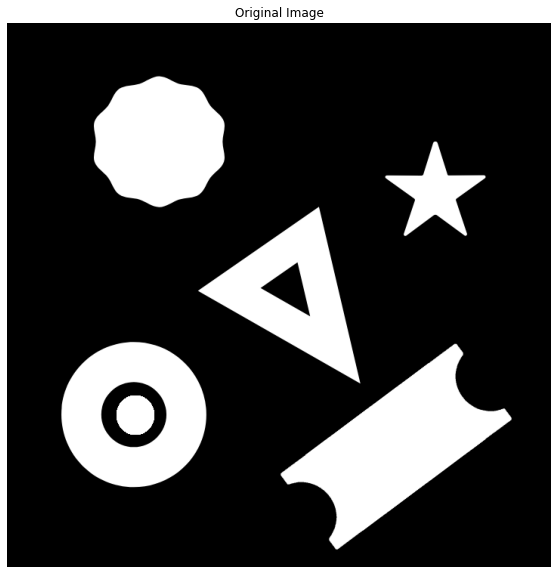
# Read the image
image1 = cv2.imread('media/image.png')

# Display the image
plt.figure(figsize=[10,10])
plt.imshow(image1[:,:,::-1]);plt.title("Original Image");plt.axis("off");
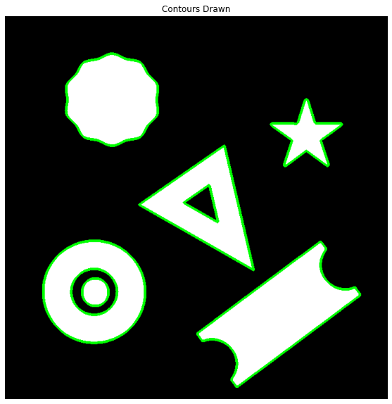
Detect and draw Contours
Next, we will detect and draw contours on the image as before using the cv2.findContours()and cv2.drawContours()
# Make a copy of the original image so it is not overwritten
image1_copy = image1.copy()

# Convert to grayscale.
image_gray = cv2.cvtColor(image1_copy,cv2.COLOR_BGR2GRAY)

# Find all contours in the image.
contours, hierarchy = cv2.findContours(image_gray, cv2.RETR_CCOMP, cv2.CHAIN_APPROX_NONE)

# Draw the selected contour
cv2.drawContours(image1_copy, contours, -1, (0,255,0), 3);

# Display the result
plt.figure(figsize=[10,10])
plt.imshow(image1_copy[:,:,::-1]);plt.axis("off");plt.title('Contours Drawn');
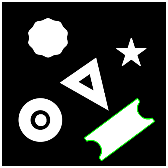
Extracting the Largest Contour in the image
When building vision applications using contours, often we are interested in retrieving the contour of the largest object in the image and discard others as noise. This can be done using the built-in python’s max() function with the contours list. The max() function takes in as input the contours list along with a key parameter which refers to the single argument function used to customize the sort order. The function is applied to each item on the iterable. So for retrieving the largest contour we use the key cv2.contourArea which is a function that returns the area of a contour. It is applied to each contour in the list and then the max() function returns the largest contour based on its area.
image1_copy = image1.copy()

# Convert to grayscale
gray_image = cv2.cvtColor(image1_copy,cv2.COLOR_BGR2GRAY)

# Find all contours in the image.
contours, hierarchy = cv2.findContours(gray_image, cv2.RETR_LIST, cv2.CHAIN_APPROX_NONE)

# Retreive the biggest contour
biggest_contour = max(contours, key = cv2.contourArea)

# Draw the biggest contour
cv2.drawContours(image1_copy, biggest_contour, -1, (0,255,0), 4);

# Display the results
plt.figure(figsize=[10,10])
plt.imshow(image1_copy[:,:,::-1]);plt.axis("off");
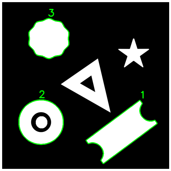
Sorting Contours in terms of size
Extracting the largest contour worked out well, but sometimes we are interested in more than one contour from a sorted list of contours. In such cases, another built-in python function sorted() can be used instead. sorted() function also takes in the optional key parameter which we use as before for returning the area of each contour. Then the contours are sorted based on area and the resultant list is returned. We also specify the order of sort reverse = True i.e in descending order of area size.
image1_copy = image1.copy()

# Convert to grayscale.
imageGray = cv2.cvtColor(image1_copy,cv2.COLOR_BGR2GRAY)

# Find all contours in the image.
contours, hierarchy = cv2.findContours(imageGray, cv2.RETR_CCOMP, cv2.CHAIN_APPROX_NONE)

# Sort the contours in decreasing order
sorted_contours = sorted(contours, key=cv2.contourArea, reverse= True)

# Draw largest 3 contours
for i, cont in enumerate(sorted_contours[:3],1):

    # Draw the contour
    cv2.drawContours(image1_copy, cont, -1, (0,255,0), 3)

    # Display the position of contour in sorted list
    cv2.putText(image1_copy, str(i), (cont[0,0,0], cont[0,0,1]-10), cv2.FONT_HERSHEY_SIMPLEX, 1.4, (0, 255, 0),4)


# Display the result
plt.figure(figsize=[10,10])
plt.imshow(image1_copy[:,:,::-1]);plt.axis("off");
Drawing a rectangle around the contour
Bounding rectangles are often used to highlight the regions of interest in the image. If this region of interest is a detected contour of a shape in the image, we can enclose it within a rectangle. There are two types of bounding rectangles that you may draw:
- Straight Bounding Rectangle
- Rotated Rectangle
For both types of bounding rectangles, their vertices are calculated using the coordinates in the contour list.
Straight Bounding Rectangle
A straight bounding rectangle is simply an upright rectangle that does not take into account the rotation of the object. Its vertices can be calculated using the cv2.boundingRect() function which calculates the vertices for the minimal up-right rectangle possible using the extreme coordinates in the contour list. The coordinates can then be drawn as rectangle using cv2.rectangle() function.
Function Syntax:
x, y, w, h = cv2.boundingRect(array)
Parameters:
array– It is the Input gray-scale image or 2D point set from which the bounding rectangle is to be created
Returns:
x– It is X-coordinate of the top-left cornery– It is Y-coordinate of the top-left cornerw– It is the width of the rectangleh– It is the height of the rectangle
image1_copy = image1.copy()

# Convert to grayscale.
gray_scale = cv2.cvtColor(image1_copy,cv2.COLOR_BGR2GRAY)

# Find all contours in the image.
contours, hierarchy = cv2.findContours(gray_scale, cv2.RETR_CCOMP, cv2.CHAIN_APPROX_NONE)

# Get the bounding rectangle
x, y, w, h = cv2.boundingRect(contours[1])

# Draw the rectangle around the object.
cv2.rectangle(image1_copy, (x, y), (x+w, y+h), (0, 255, 0), 3)

# Display the result
plt.figure(figsize=[10,10])
plt.imshow(image1_copy[:,:,::-1]);plt.axis("off");
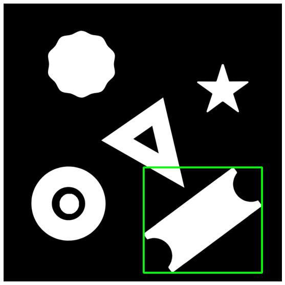
However, the bounding rectangle created is not a minimum area bounding rectangle often causing it to overlap with any other objects in the image. But what if the rectangle is rotated so that the area can be minimized to tightly fit the shape.
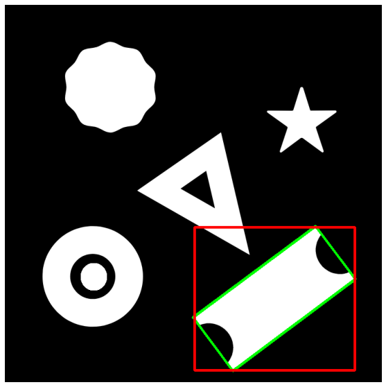
Rotated Rectangle
As the name suggests the rectangle drawn is rotated at an angle so that the area it occupies to enclose the contour is minimum. The function you can use to calculate the vertices of the rotated rectangle is cv2.minAreaRect(), which uses the contour point set to calculate the coordinates of the top left corner of the rectangle, its width, height, and the angle of rotation of the rectangle.
Function Syntax:
retval = cv2.minAreaRect(points)
Parameters:
array– It is the Input gray-scale image or 2D point set from which the bounding rectangle is to be created
Returns:
retval– A tuple consisting of:- x,y coordinates of the top-left vertex
- width, height of the rectangle
- angle of rotation of the rectangle
Since the cv2.rectangle() function can only draw up-right rectangles we cannot use it to draw the rotated rectangle. Instead, we can calculate the 4 vertices of the rectangle using the cv2.boxPoints() function which takes the rect tuple as input. Once we have the vertices, the rectangle can be simply drawn using the cv2.drawContours() function.
image1_copy = image1.copy()

# Convert to grayscale
gray_scale = cv2.cvtColor(image1_copy,cv2.COLOR_BGR2GRAY)

# Find all contours in the image
contours, hierarchy = cv2.findContours(gray_scale, cv2.RETR_CCOMP, cv2.CHAIN_APPROX_NONE)

# calculate the minimum area Bounding rect
rect = cv2.minAreaRect(contours[1])

# Check out the rect object
print(rect)

# convert the rect object to box points
box =  cv2.boxPoints(rect).astype('int')

# Draw a rectangle around the object
cv2.drawContours(image1_copy,
					,0,(0,255,0),3)

# Display the results
plt.figure(figsize=[10,10])
plt.imshow(image1_copy[:,:,::-1]);plt.axis("off");rect: ((514.5311279296875, 560.094482421875), (126.98052215576172, 291.55517578125), 53.310279846191406)
rect: ((514.5311279296875, 560.094482421875), (126.98052215576172, 291.55517578125), 53.310279846191406)

The four corner points that formed the contour for our the rotated rectangle:
box
array([[359, 596],
[593, 422],
[669, 523],
[435, 698]])
This is the minimum area bounding rectangle possible. Let’s see how it compares to the straight bounding box.
# Draw the up-right rectangle
cv2.rectangle(image1_copy, (x, y), (x+w, y+h), (0,0, 255), 3)

# Display the result
plt.figure(figsize=[10,10])
plt.imshow(image1_copy[:,:,::-1]);plt.axis("off");
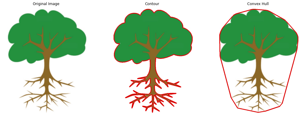
Drawing Convex Hull
A convex hull is another useful way to represent the contour onto the image. The function cv2.convexHull() checks a curve for convexity defects and corrects it. Convex curves are curves that are bulged out. And if it is bulged inside (Concave), it is called convexity defects.
Finding the convex hull of a contour can be very useful when working with shape matching techniques. This is because the convex hull of a contour highlights its prominent features while discarding smaller variations in the shape.
Function Syntax:
hull = cv2.convexHull(points, hull, clockwise, returnPoints)
Parameters:
points– Input 2D point set. This is a single contour.clockwise– Orientation flag. If it is true, the output convex hull is oriented clockwise. Otherwise, it is oriented counter-clockwise. The assumed coordinate system has its X axis pointing to the right, and its Y axis pointing upwards.returnPoints– Operation flag. In case of a matrix, when the flag is true, the function returns convex hull points. Otherwise, it returns indices of the convex hull points. By default it is True.
Returns:
hull– Output convex hull. It is either an integer vector of indices or vector of points. In the first case, the hull elements are 0-based indices of the convex hull points in the original array (since the set of convex hull points is a subset of the original point set). In the second case, hull elements are the convex hull points themselves.
image2 = cv2.imread('media/tree.jpg')

hull_img = image2.copy()
contour_img = image2.copy()

# Convert the image to gray-scale
gray = cv2.cvtColor(image2, cv2.COLOR_BGR2GRAY)

# Create a binary thresholded image
_, binary = cv2.threshold(gray, 230, 255, cv2.THRESH_BINARY_INV)

# Find the contours from the thresholded image
contours, hierarchy = cv2.findContours(binary, cv2.RETR_EXTERNAL, cv2.CHAIN_APPROX_SIMPLE)

# Since the image only has one contour, grab the first contour
cnt = contours[0]

# Get the required hull
hull = cv2.convexHull(cnt)

# draw the hull
cv2.drawContours(hull_img, [hull], 0 , (0,0,220), 3)

# draw the contour
cv2.drawContours(contour_img, [cnt], 0, (0,0,220), 3)

plt.figure(figsize=[18,18])
plt.subplot(131);plt.imshow(image2[:,:,::-1]);plt.title("Original Image");plt.axis('off')
plt.subplot(132);plt.imshow(contour_img[:,:,::-1]);plt.title("Contour");plt.axis('off');
plt.subplot(133);plt.imshow(hull_img[:,:,::-1]);plt.title("Convex Hull");plt.axis('off');
[optin-monster slug=”d8wgq6fdm5mppdb5fi99″]
Summary
In today’s post, we familiarized ourselves with many of the contour manipulation techniques. These manipulations help make contour detection an even more useful tool applicable to a wider variety of problems
We saw how you can filter out contours based on their size using the built-in max() and sorted() functions, allowing you to extract the largest contour or a list of contours sorted by size.
Then we learned how you can highlight contour detections with bounding rectangles of two types, the straight bounding rectangle and the rotated one.
Lastly, we learned about convex hulls and how you can find them for detected contours. A very handy technique that can prove to be useful for object detection with shape matching.
This sums up the second post in the series. In the next post, we’re going to learn various analytical techniques to analyze contours in order to classify and distinguish between different Objects.
So if you found this lesson useful, let me know in the comments and you can also support me and the Bleed AI team on patreon here.
If you need 1 on 1 Coaching in AI/computer vision regarding your project, or your career then you reach out to me personally here


0 Comments