Watch Video Here
In the previous tutorial of this series, we learned how the mouse events and trackbars work in OpenCV, we went into all the details needed for you to get comfortable with using these. Now in this tutorial, we will learn to create a user interface similar to the Instagram filter selection screen using mouse events & trackbars in OpenCV.
But first, we will learn what LookUp Tables are, why are they preferred along with their use cases in real-life, and then utilize these LookUp Tables to create some spectacular photo effects called Color Filters a.k.a. Tone Effects.

This Tutorial is built on top of the previous one so if you haven’t read the previous post and don’t know how to use mouse events and trackbars in OpenCV, then you can read that post here. As we are gonna utilize trackbars to control the intensities of the filters and mouse events to select a Color filter to apply.
This is the second tutorial in our 3 part Creating Instagram Filters series (in which we will learn to create some interesting and famous Instagram filters-like effects). All three posts are titled as:
- Part 1: Working With Mouse & Trackbar Events in OpenCV
- Part 2: Working With Lookup Tables & Applying Color Filters on Images & Videos (Current tutorial)
- Part 3: Designing Advanced Image Filters in OpenCV
Download Code:
Outline
The tutorial is divided into the following parts:
Alright, without further ado, let’s dive in.
Import the Libraries
First, we will import the required libraries.
|
1 2 3 |
import cv2 import numpy as np import matplotlib.pyplot as plt |
Introduction to LookUp Tables
LookUp Tables (also known as LUTs) in OpenCV are arrays containing a mapping of input values to output values that allow replacing computationally expensive operations with a simpler array indexing operation at run-time.* Don’t worry in case the definition felt like mumbo-jumbo to you, I am gonna break down this to you in a very digestible and intuitive manner. Check the image below containing a LookUp Table of Square operation.
So it’s just a mapping of a bunch of input values to their corresponding outputs i.e., normally outcomes of a certain operation (like square in the image above) on the input values. These are structured in an array containing the output mapping values at the indexes equal to the input values. Meaning the output for the input value 2 will be at the index 2 in the array, and i.e., 4 in the image above. Now that we know what exactly these LookUp Tables are, so let’s move to create one for the square operation.
|
1 2 3 4 5 6 7 8 9 10 11 12 13 14 15 |
# Initialize a list to store the LookUpTable mapping. square_table = [] # Iterate over 100 times. # We are creating mapping only for input values [0-99]. for i in range(100): # Take Square of the i and append it into the list. square_table.append(pow(i, 2)) # Convert the list into an array. square_table = np.array(square_table) # Display first ten elements of the lookUp table. print(f'First 10 mappings: {square_table[:10]}') |
First 10 mappings: [ 0 1 4 9 16 25 36 49 64 81]
This is how a LookUp Table is created, yes it’s that simple. But you may be thinking how and for what are they used for? Well as mentioned in the definition, these are used to replace computationally expensive operations (in our example, Square) with a simpler array indexing operation at run-time.
So in simple words instead of calculating the results at run-time, these allow to transform input values into their corresponding outputs by looking up in the mapping table by doing something like this:
|
1 2 3 4 5 |
# Set the input value to get its square from the LookUp Table. input_value = 10 # Display the output value returned from the LookUp Table. print(f'Square of {input_value} is: {square_table[input_value]}') |
Square of 10 is: 100
This eliminates the need of performing a computationally expensive operation at run-time as long as the input values have a limited range which is always true for images as they have pixels intensities [0-255].
Almost all the image processing operations can be performed much more efficiently using these LookUp Tables like increasing/decreasing image brightness, saturation, contrast, even changing specific colors in images like the black and white color shift done in the image below.
Stunning! right? let’s try to perform this color shift on a few sample images. First, we will construct a LookUp Table mapping all the pixel values greater than 220 (white) to 0 (black) and then transform an image according to the lookup table using the cv2.LUT() function.
Function Syntax:
Parameters:
src:– It is the input array (image) of 8-bit elements.lut:– It is the look-up table of 256 elements.
Returns:
dst:– It is the output array of the same size and number of channels as src, and the same depth as lut.
Note: In the case of a multi-channel input array (src), the table (lut) should either have a single channel (in this case the same table is used for all channels) or the same number of channels as in the input array (src).
|
1 2 3 4 5 6 7 8 9 10 11 12 13 14 15 16 17 18 19 20 21 22 23 24 25 26 27 28 29 30 31 |
# Read a sample image. image = cv2.imread('media/sample.jpg') # Initialize a list to store the lookuptable mapping. white_to_black_table = [] # Iterate over 256 times. # As images have pixels intensities [0-255]. for i in range(256): # Check if i is greater than 220. if i > 220: # Append 0 into the list. # This will convert pixels > 220 to 0. white_to_black_table.append(0) # Otherwise. else: # Append i into the list. # The pixels <= 220 will remain the same. white_to_black_table.append(i) # Transform the image according to the lookup table. output_image = cv2.LUT(image, np.array(white_to_black_table).astype("uint8")) # Display the original sample image and the resultant image. plt.figure(figsize=[15,15]) plt.subplot(121);plt.imshow(image[:,:,::-1]);plt.title("Sample Image");plt.axis('off'); plt.subplot(122);plt.imshow(output_image[:,:,::-1]);plt.title("Output Image");plt.axis('off'); |
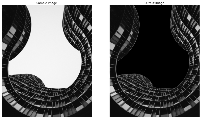
As you can see it worked as expected. Now let’s construct another LookUp Table mapping all the pixel values less than 50 (black) to 255 (white) and then transform another sample image to switch the black color in the image with white.
|
1 2 3 4 5 6 7 8 9 10 11 12 13 14 15 16 17 18 19 20 21 22 23 24 25 26 27 28 |
# Read another sample image. image = cv2.imread('media/wall.jpg') # Initialize a list to store the lookuptable mapping. black_to_white_table = [] # Iterate over 256 times. for i in range(256): # Check if i is less than 50. if i < 50: # Append 255 into the list. black_to_white_table.append(255) # Otherwise. else: # Append i into the list. black_to_white_table.append(i) # Transform the image according to the lookup table. output_image = cv2.LUT(image, np.array(black_to_white_table).astype("uint8")) # Display the original sample image and the resultant image. plt.figure(figsize=[15,15]) plt.subplot(121);plt.imshow(image[:,:,::-1]);plt.title("Sample Image");plt.axis('off'); plt.subplot(122);plt.imshow(output_image[:,:,::-1]);plt.title("Output Image");plt.axis('off'); |
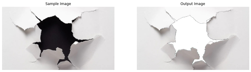
The Black to white shift is also working perfectly fine. You can perform a similar shift with any color you want and this technique can be really helpful in efficiently changing green background screens from high-resolution videos and creating some interesting effects.
But we still don’t have an idea how much computational power and time these LookUp Tables save and are they worth trying? Well, this completely depends upon your use case, the number of images you want to transform, the resolution of the images you are working on, etc.
How about we perform a black to white shift on a few images with and without LookUp Tables and note the execution time to get an idea of the time difference? You can change the number of images and their resolution according to your use case.
|
1 2 3 |
# Set the number of images and their resolution. num_of_images = 100 image_resolution = (960, 1280) |
First, let’s do it without using LookUp Tables.
|
1 2 3 4 5 6 7 8 9 10 11 |
%%time # Use magic command to measure execution time. # Iterate over the number of times equal to the number of images. for i in range(num_of_images): # Create a dummy image with each pixel value equal to 0. image = np.zeros(shape=image_resolution, dtype=np.uint8) # Convert pixels < 50 to 255. image[image<50] = 255 |
Wall time: 194 ms
We have the execution time without using LookUp Tables, now let’s check the difference by performing the same operation utilizing LookUp Tables. First we will create the look up Table, this only has to be done once.
|
1 2 3 4 5 6 7 8 9 10 11 12 13 14 15 16 17 |
# Initialize a list to store the lookuptable mapping. table = [] # Iterate over 256 times. for i in range(256): # Check if i is less than 50. if i < 50: # Append 255 into the list. table.append(255) # Otherwise. else: # Append i into the list. table.append(i) |
Now we’ll use the look up table created above in action
|
1 2 3 4 5 6 7 8 9 10 11 |
%%time # Use magic command to measure execution time. # Iterate over the number of times equal to the number of images. for i in range(num_of_images): # Create a dummy image with each pixel value equal to 0. image = np.zeros(shape=image_resolution, dtype=np.uint8) # Transform the image according to the lookup table. cv2.LUT(image, np.array(table).astype("uint8")) |
Wall time: 81.2 ms
So the time taken in the second approach (LookUp Tables) is significantly lesser while the results are the same.
Applying Color Filters on Images/Videos
Finally comes the fun part, Color Filters that give interesting lighting effects to images, simply by modifying pixel values of different color channels (R,G,B) of images and we will create some of these effects utilizing LookUp tables.
We will first construct a lookup table, containing the mapping that we will need to apply different color filters.
|
1 2 3 4 5 6 7 8 9 10 |
# Initialize a list to store the lookuptable for the color filter. color_table = [] # Iterate over 128 times from 128-255. for i in range(128, 256): # Extend the table list and add the i two times in the list. # We want to increase pixel intensities that's why we are adding only values > 127. # We are adding same value two times because we need total 256 elements in the list. color_table.extend([i, i]) |
|
1 2 |
# We just added each element 2 times. print(color_table[:10], "Length of table: " + str(len(color_table))) |
[128, 128, 129, 129, 130, 130, 131, 131, 132, 132] Length of table: 256
Now we will create a function applyColorFilter() that will utilize the lookup table we created above, to increase pixel intensities of specified channels of images and videos and will display the resultant image along with the original image or return the resultant image depending upon the passed arguments.
|
1 2 3 4 5 6 7 8 9 10 11 12 13 14 15 16 17 18 19 20 21 22 23 24 25 26 27 28 29 30 31 32 33 34 35 36 37 38 |
def applyColorFilter(image, channels_indexes, display=True): ''' This function will apply different interesting color lighting effects on an image. Args: image: The image on which the color filter is to be applied. channels_indexes: A list of channels indexes that are required to be transformed. display: A boolean value that is if set to true the function displays the original image, and the output image with the color filter applied and returns nothing. Returns: output_image: The transformed resultant image on which the color filter is applied. ''' # Access the lookuptable containing the mapping we need. global color_table # Create a copy of the image. output_image = image.copy() # Iterate over the indexes of the channels to modify. for channel_index in channels_indexes: # Transform the channel of the image according to the lookup table. output_image[:,:,channel_index] = cv2.LUT(output_image[:,:,channel_index], np.array(color_table).astype("uint8")) # Check if the original input image and the resultant image are specified to be displayed. if display: # Display the original input image and the resultant image. plt.figure(figsize=[15,15]) plt.subplot(121);plt.imshow(image[:,:,::-1]);plt.title("Sample Image");plt.axis('off'); plt.subplot(122);plt.imshow(output_image[:,:,::-1]);plt.title("Output Image");plt.axis('off'); # Otherwise else: # Return the resultant image. return output_image |
Now we will utilize the function applyColorFilter() to apply different color effects on a few sample images and display the results.
|
1 2 3 |
# Read a sample image and apply color filter on it. image = cv2.imread('media/sample1.jpg') applyColorFilter(image, channels_indexes=[0]) |
|
1 2 3 |
# Read another sample image and apply color filter on it. image = cv2.imread('media/sample2.jpg') applyColorFilter(image, channels_indexes=[1]) |
|
1 2 3 |
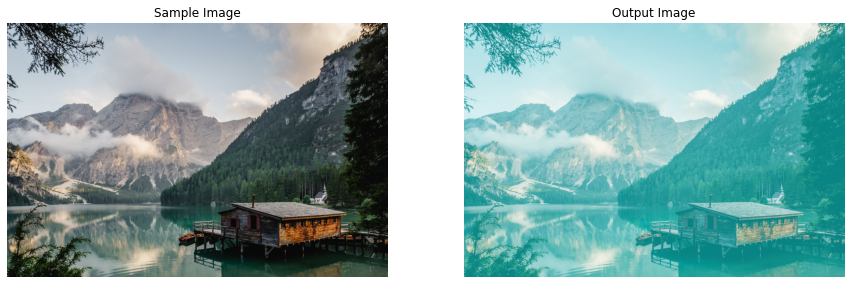
# Read another sample image and apply color filter on it. image = cv2.imread('media/sample3.jpg') applyColorFilter(image, channels_indexes=[2]) |
|
1 2 3 |
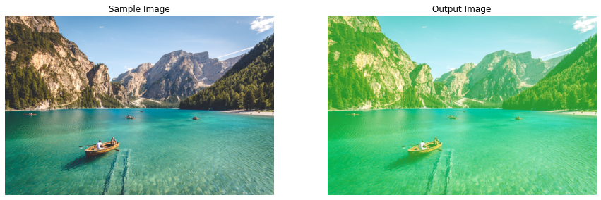
# Read another sample image and apply color filter on it. image = cv2.imread('media/sample4.jpg') applyColorFilter(image, channels_indexes=[0, 1]) |
|
1 2 3 |
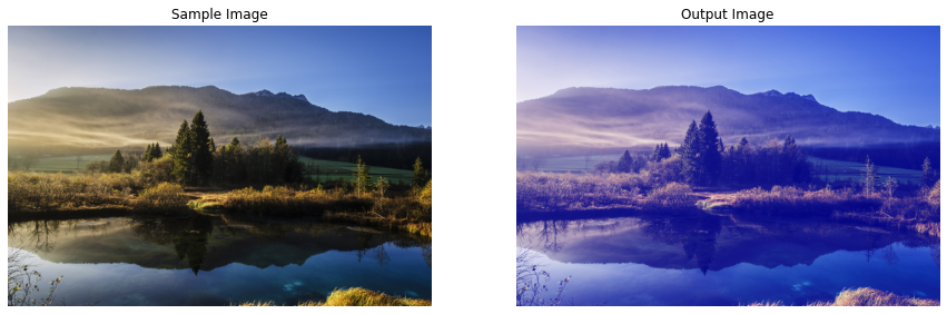
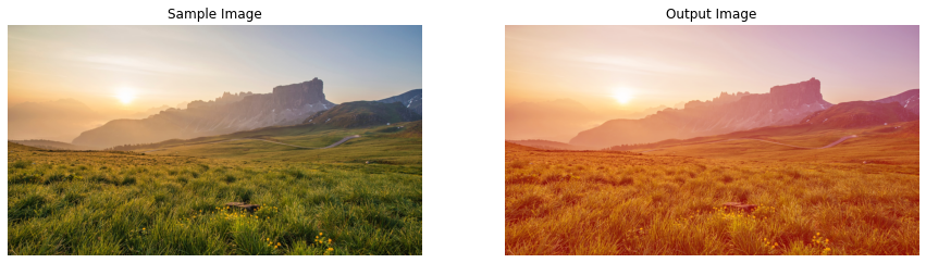
# Read another sample image and apply color filter on it. image = cv2.imread('media/sample5.jpg') applyColorFilter(image, channels_indexes=[0, 2]) |
Cool! right? the results are astonishing but some of them are feeling a bit too much. So how about we will create another function changeIntensity() to control the intensity of these filters, again by utilizing LookUpTables. The function will simply increase or decrease the pixel intensities of the same color channels that were modified by the applyColorFilter() function and will display the results or return the resultant image depending upon the passed arguments.
For modifying the pixel intensities we will use the Gamma Correction technique, also known as the Power Law Transform. Its a nonlinear operation normally used to correct the brightness of an image using the following equation:
O=(I255)γ×255
Here γ<1 will increase the pixel intensities while γ>1 will decrease the pixel intensities and the filter effect. To perform the process, we will first construct a lookup table using the equation above.
|
1 2 3 4 5 6 7 8 9 10 11 12 13 |
# Initialize a variable to store previous gamma value. prev_gamma = 1.0 # Initialize a list to store the lookuptable for the change intensity operation. intensity_table = [] # Iterate over 256 times. for i in range(256): # Calculate the mapping output value for the i input value, # and clip (limit) the values between 0 and 255. # Also append it into the look-up table list. intensity_table.append(np.clip(a=pow(i/255.0, prev_gamma)*255.0, a_min=0, a_max=255)) |
And then we will create the changeIntensity() function, which will use the table we have constructed and will re-construct the table every time the gamma value changes.
|
1 2 3 4 5 6 7 8 9 10 11 12 13 14 15 16 17 18 19 20 21 22 23 24 25 26 27 28 29 30 31 32 33 34 35 36 37 38 39 40 41 42 43 44 45 46 47 48 49 50 51 52 53 54 55 56 57 58 59 60 61 62 |
def changeIntensity(image, scale_factor, channels_indexes, display=True): ''' This function will change intensity of the color filters. Args: image: The image on which the color filter intensity is required to be changed. scale_factor: A number that will be used to calculate the required gamma value. channels_indexes: A list of indexes of the channels on which the color filter was applied. display: A boolean value that is if set to true the function displays the original image, and the output image, and returns nothing. Returns: output_image: A copy of the input image with the color filter intensity changed. ''' # Access the previous gamma value and the table contructed # with the previous gamma value. global prev_gamma, intensity_table # Create a copy of the input image. output_image = image.copy() # Calculate the gamma value from the passed scale factor. gamma = 1.0/scale_factor # Check if the previous gamma value is not equal to the current gamma value. if gamma != prev_gamma: # Update the intensity lookuptable to an empty list. # We will have to re-construct the table for the new gamma value. intensity_table = [] # Iterate over 256 times. for i in range(256): # Calculate the mapping output value for the i input value # And clip (limit) the values between 0 and 255. # Also append it into the look-up table list. intensity_table.append(np.clip(a=pow(i/255.0, gamma)*255.0, a_min=0, a_max=255)) # Update the previous gamma value. prev_gamma = gamma # Iterate over the indexes of the channels. for channel_index in channels_indexes: # Change intensity of the channel of the image according to the lookup table. output_image[:,:,channel_index] = cv2.LUT(output_image[:,:,channel_index], np.array(intensity_table).astype("uint8")) # Check if the original input image and the output image are specified to be displayed. if display: # Display the original input image and the output image. plt.figure(figsize=[15,15]) plt.subplot(121);plt.imshow(image[:,:,::-1]);plt.title("Color Filter");plt.axis('off'); plt.subplot(122);plt.imshow(output_image[:,:,::-1]);plt.title("Color Filter with Modified Intensity") plt.axis('off') # Otherwise. else: # Return the output image. return output_image |
Now let’s check how the changeIntensity() function works on a few sample images.
|
1 2 3 4 |
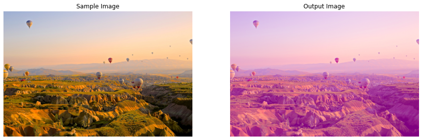
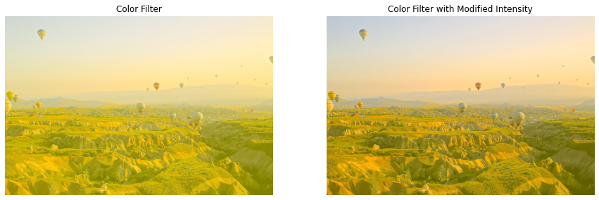
# Read a sample image and apply color filter on it with intensity 0.6. image = cv2.imread('media/sample5.jpg') image = applyColorFilter(image, channels_indexes=[1, 2], display=False) changeIntensity(image, scale_factor=0.6, channels_indexes=[1, 2]) |
|
1 2 3 4 |
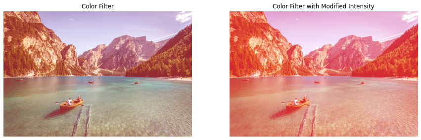
# Read another sample image and apply color filter on it with intensity 3. image = cv2.imread('media/sample2.jpg') image = applyColorFilter(image, channels_indexes=[2], display=False) changeIntensity(image, scale_factor=3, channels_indexes=[2]) |
Apply Color Filters On Real-Time Web-cam Feed
The results on the images are exceptional, now let’s check how these filters will look on a real-time webcam feed. But first, we will create a mouse event callback function selectFilter(), that will allow us to select the filter to apply by clicking on the filter preview on the top of the frame in real-time.
|
1 2 3 4 5 6 7 8 9 10 11 12 13 14 15 16 17 18 19 20 21 22 23 24 25 26 27 28 29 30 31 32 33 34 35 36 37 38 39 40 41 42 43 44 45 46 47 48 49 50 51 52 53 54 55 56 57 58 59 60 61 62 63 64 65 66 67 68 69 70 71 72 73 74 75 76 77 78 79 80 81 82 83 84 85 86 87 88 89 90 91 92 93 94 95 96 |
def selectFilter(event, x, y, flags, userdata): ''' This function will update the current filter applied on the frame based on different mouse events. Args: event: The mouse event that is captured. x: The x-coordinate of the mouse pointer position on the window. y: The y-coordinate of the mouse pointer position on the window. flags: It is one of the MouseEventFlags constants. userdata: The parameter passed from the `cv2.setMouseCallback()` function. ''' # Access the filter applied and the channels indexes variable. global filter_applied, channels_indexes # Check if the left mouse button is pressed. if event == cv2.EVENT_LBUTTONDOWN: # Check if the mouse pointer y-coordinate is less than equal to a certain threshold. if y <= 10+preview_height: # Check if the mouse pointer x-coordinate is over the Blue filter ROI. if x > (int(frame_width//1.25)-preview_width//2) and \ x < (int(frame_width//1.25)-preview_width//2)+preview_width: # Update the filter applied variable value to Blue. filter_applied = 'Blue' # Update the channels indexes list to store the # indexes of the channels to modify for the Blue filter. channels_indexes = [0] # Check if the mouse pointer x-coordinate is over the Green filter ROI. elif x>(int(frame_width//1.427)-preview_width//2) and \ x<(int(frame_width//1.427)-preview_width//2)+preview_width: # Update the filter applied variable value to Green. filter_applied = 'Green' # Update the channels indexes list to store the # indexes of the channels to modify for the Green filter. channels_indexes = [1] # Check if the mouse pointer x-coordinate is over the Red filter ROI. elif x>(frame_width//1.665-preview_width//2) and \ x<(frame_width//1.665-preview_width//2)+preview_width: # Update the filter applied variable value to Red. filter_applied = 'Red' # Update the channels indexes list to store the # indexes of the channels to modify for the Red filter. channels_indexes = [2] # Check if the mouse pointer x-coordinate is over the Normal frame ROI. elif x>(int(frame_width//2)-preview_width//2) and \ x<(int(frame_width//2)-preview_width//2)+preview_width: # Update the filter applied variable value to Normal. filter_applied = 'Normal' # Update the channels indexes list to empty list. # As no channels are modified in the Normal filter. channels_indexes = [] # Check if the mouse pointer x-coordinate is over the Cyan filter ROI. elif x>(int(frame_width//2.5)-preview_width//2) and \ x<(int(frame_width//2.5)-preview_width//2)+preview_width: # Update the filter applied variable value to Cyan Filter. filter_applied = 'Cyan' # Update the channels indexes list to store the # indexes of the channels to modify for the Cyan filter. channels_indexes = [0, 1] # Check if the mouse pointer x-coordinate is over the Purple filter ROI. elif x>(int(frame_width//3.33)-preview_width//2) and \ x<(int(frame_width//3.33)-preview_width//2)+preview_width: # Update the filter applied variable value to Purple. filter_applied = 'Purple' # Update the channels indexes list to store the # indexes of the channels to modify for the Purple filter. channels_indexes = [0, 2] # Check if the mouse pointer x-coordinate is over the Yellow filter ROI. elif x>(int(frame_width//4.99)-preview_width//2) and \ x<(int(frame_width//4.99)-preview_width//2)+preview_width: # Update the filter applied variable value to Yellow. filter_applied = 'Yellow' # Update the channels indexes list to store the # indexes of the channels to modify for the Yellow filter. channels_indexes = [1, 2] |
Now without further ado, let’s test the filters on a real-time webcam feed, we will be switching between the filters by utilizing the selectFilter() function created above and will use a trackbar to change the intensity of the filter applied in real-time.
|
1 2 3 4 5 6 7 8 9 10 11 12 13 14 15 16 17 18 19 20 21 22 23 24 25 26 27 28 29 30 31 32 33 34 35 36 37 38 39 40 41 42 43 44 45 46 47 48 49 50 51 52 53 54 55 56 57 58 59 60 61 62 63 64 65 66 67 68 69 70 71 72 73 74 75 76 77 78 79 80 81 82 83 84 85 86 87 88 89 90 91 92 93 94 95 96 97 98 99 100 101 102 103 104 105 106 107 108 109 110 111 112 113 114 115 116 117 118 119 120 121 122 123 124 125 126 127 128 129 130 131 132 133 134 135 136 137 138 139 140 141 142 143 144 145 146 147 148 149 150 151 152 153 154 155 156 157 |
# Initialize the VideoCapture object to read from the webcam. camera_video = cv2.VideoCapture(0) camera_video.set(3,1280) camera_video.set(4,960) # Create a named resizable window. cv2.namedWindow('Color Filters', cv2.WINDOW_NORMAL) # Create the function for the trackbar since its mandatory. def nothing(x): pass # Create trackbar named Intensity with the range [0-100]. cv2.createTrackbar('Intensity', 'Color Filters', 50, 100, nothing) # Attach the mouse callback function to the window. cv2.setMouseCallback('Color Filters', selectFilter) # Initialize a variable to store the current applied filter. filter_applied = 'Normal' # Initialize a list to store the indexes of the channels # that were modified to apply the current filter. # This list will be required to change intensity of the applied filter. channels_indexes = [] # Iterate until the webcam is accessed successfully. while camera_video.isOpened(): # Read a frame. ok, frame = camera_video.read() # Check if frame is not read properly then # continue to the next iteration to read the next frame. if not ok: continue # Flip the frame horizontally for natural (selfie-view) visualization. frame = cv2.flip(frame, 1) # Get the height and width of the frame of the webcam video. frame_height, frame_width, _ = frame.shape # Initialize a dictionary and store the copies of the frame with the # filters applied by transforming some different channels combinations. filters = {'Normal': frame.copy(), 'Blue': applyColorFilter(frame, channels_indexes=[0], display=False), 'Green': applyColorFilter(frame, channels_indexes=[1], display=False), 'Red': applyColorFilter(frame, channels_indexes=[2], display=False), 'Cyan': applyColorFilter(frame, channels_indexes=[0, 1], display=False), 'Purple': applyColorFilter(frame, channels_indexes=[0, 2], display=False), 'Yellow': applyColorFilter(frame, channels_indexes=[1, 2], display=False)} # Initialize a list to store the previews of the filters. filters_previews = [] # Iterate over the filters dictionary. for filter_name, filter_applied_frame in filters.items(): # Check if the filter we are iterating upon, is applied. if filter_applied == filter_name: # Set color to green. # This will be the border color of the filter preview. # And will be green for the filter applied and white for the other filters. color = (0,255,0) # Otherwise. else: # Set color to white. color = (255,255,255) # Make a border around the filter we are iterating upon. filter_preview = cv2.copyMakeBorder(src=filter_applied_frame, top=100, bottom=100, left=10, right=10, borderType=cv2.BORDER_CONSTANT, value=color) # Resize the filter applied frame to the 1/10th of its current width # while keeping the aspect ratio constant. filter_preview = cv2.resize(filter_preview, (frame_width//10, int(((frame_width//10)/frame_width)*frame_height))) # Append the filter preview into the list. filters_previews.append(filter_preview) # Update the frame with the currently applied Filter. frame = filters[filter_applied] # Get the value of the filter intensity from the trackbar. filter_intensity = cv2.getTrackbarPos('Intensity', 'Color Filters')/100 + 0.5 # Check if the length of channels indexes list is > 0. if len(channels_indexes) > 0: # Change the intensity of the applied filter. frame = changeIntensity(frame, filter_intensity, channels_indexes, display=False) # Get the new height and width of the previews. preview_height, preview_width, _ = filters_previews[0].shape # Overlay the resized preview filter images over the frame by updating # its pixel values in the region of interest. ####################################################################################### # Overlay the Blue Filter preview on the frame. frame[10: 10+preview_height, (int(frame_width//1.25)-preview_width//2):\ (int(frame_width//1.25)-preview_width//2)+preview_width] = filters_previews[1] # Overlay the Green Filter preview on the frame. frame[10: 10+preview_height, (int(frame_width//1.427)-preview_width//2):\ (int(frame_width//1.427)-preview_width//2)+preview_width] = filters_previews[2] # Overlay the Red Filter preview on the frame. frame[10: 10+preview_height, (int(frame_width//1.665)-preview_width//2):\ (int(frame_width//1.665)-preview_width//2)+preview_width] = filters_previews[3] # Overlay the normal frame (no filter) preview on the frame. frame[10: 10+preview_height, (frame_width//2-preview_width//2):\ (frame_width//2-preview_width//2)+preview_width] = filters_previews[0] # Overlay the Cyan Filter preview on the frame. frame[10: 10+preview_height, (int(frame_width//2.5)-preview_width//2):\ (int(frame_width//2.5)-preview_width//2)+preview_width] = filters_previews[4] # Overlay the Purple Filter preview on the frame. frame[10: 10+preview_height, (int(frame_width//3.33)-preview_width//2):\ (int(frame_width//3.33)-preview_width//2)+preview_width] = filters_previews[5] # Overlay the Yellow Filter preview on the frame. frame[10: 10+preview_height, (int(frame_width//4.99)-preview_width//2):\ (int(frame_width//4.99)-preview_width//2)+preview_width] = filters_previews[6] ####################################################################################### # Display the frame. cv2.imshow('Color Filters', frame) # Wait for 1ms. If a key is pressed, retreive the ASCII code of the key. k = cv2.waitKey(1) & 0xFF # Check if 'ESC' is pressed and break the loop. if(k == 27): break # Release the VideoCapture Object and close the windows. camera_video.release() cv2.destroyAllWindows() |
Output Video:
As expected, the results are fascinating on videos as well.
Assignment (Optional)
Apply a different color filter on the foreground and a different color filter on the background, and share the results with me in the comments section. You can use MediaPipe’s Selfie Segmentation solution to segment yourself in order to differentiate the foreground and the background.
And I have made something similar in our latest course Computer Vision For Building Cutting Edge Applications too, by Combining Emotion Recognition with AI Filters, so do check that out, if you are interested in building complex, real-world and thrilling AI applications.
Join My Course Computer Vision For Building Cutting Edge Applications Course

The only course out there that goes beyond basic AI Applications and teaches you how to create next-level apps that utilize physics, deep learning, classical image processing, hand and body gestures. Don’t miss your chance to level up and take your career to new heights
You’ll Learn about:
- Creating GUI interfaces for python AI scripts.
- Creating .exe DL applications
- Using a Physics library in Python & integrating it with AI
- Advance Image Processing Skills
- Advance Gesture Recognition with Mediapipe
- Task Automation with AI & CV
- Training an SVM machine Learning Model.
- Creating & Cleaning an ML dataset from scratch.
- Training DL models & how to use CNN’s & LSTMS.
- Creating 10 Advance AI/CV Applications
- & More
Whether you’re a seasoned AI professional or someone just looking to start out in AI, this is the course that will teach you, how to Architect & Build complex, real world and thrilling AI applications
Summary
Today, in this tutorial, we went over every bit of detail about the LookUp Tables, we learned what these LookUp Tables are, why they are useful and the use cases in which you should prefer them. Then we used these LookUp Tables to create different lighting effects (called Color Filters) on images and videos.
We utilized the concepts we learned about the Mouse Events and TrackBars in the previous tutorial of the series to switch between filters from the available options and change the applied filter intensity in real-time. Now in the next and final tutorial of the series, we will create some famous Instagram filters, so stick around for that.
And keep in mind that our intention was to teach you these crucial image processing concepts so that’s why we went for building the whole application using OpenCV (to keep the tutorial simple) but I do not think we have done justice with the user interface part, there’s room for a ton of improvements.
There are a lot of GUI libraries like PyQt, Pygame, and Kivi (to name a few) that you can use in order to make the UI more appealing for this application.
In fact, I have covered some basics of PyQt in our latest course Computer Vision For Building Cutting Edge Applications too, by creating a GUI (.exe) application to wrap up different face analysis models in a nice-looking user-friendly Interface, so if you are interested you can join this course to learn Productionizing AI Models with GUI & .exe format and a lot more. To productize any CV project, packaging is the key, and you’ll learn to do just that in my course above.


0 Comments