In the previous tutorial of this series, we learned how the mouse events and trackbars work in OpenCV, we went into all the details needed for you to get comfortable with using these. Now in this tutorial, we will learn to create a user interface similar to the Instagram filter selection screen using mouse events & trackbars in OpenCV.
But first, we will learn what LookUp Tables are, why are they preferred along with their use cases in real-life, and then utilize these LookUp Tables to create some spectacular photo effects called Color Filters a.k.a. Tone Effects.
This Tutorial is built on top of the previous one so if you haven’t read the previous post and don’t know how to use mouse events and trackbars in OpenCV, then you can read that post here. As we are gonna utilize trackbars to control the intensities of the filters and mouse events to select a Color filter to apply.
This is the second tutorial in our 3 part Creating Instagram Filters series (in which we will learn to create some interesting and famous Instagram filters-like effects). All three posts are titled as:
import cv2
import numpy as np
import matplotlib.pyplot as plt
Introduction to LookUp Tables
LookUp Tables (also known as LUTs) in OpenCV are arrays containing a mapping of input values to output values that allow replacing computationally expensive operations with a simpler array indexing operation at run-time.* Don’t worry in case the definition felt like mumbo-jumbo to you, I am gonna break down this to you in a very digestible and intuitive manner. Check the image below containing a LookUp Table of Square operation.
So it’s just a mapping of a bunch of input values to their corresponding outputs i.e., normally outcomes of a certain operation (like square in the image above) on the input values. These are structured in an array containing the output mapping values at the indexes equal to the input values. Meaning the output for the input value 2 will be at the index 2 in the array, and i.e., 4 in the image above. Now that we know what exactly these LookUp Tables are, so let’s move to create one for the square operation.
# Initialize a list to store the LookUpTable mapping.
square_table = []

# Iterate over 100 times.
# We are creating mapping only for input values [0-99].
for i in range(100):

    # Take Square of the i and append it into the list.
    square_table.append(pow(i, 2))

# Convert the list into an array.
square_table = np.array(square_table)

# Display first ten elements of the lookUp table.
print(f'First 10 mappings: {square_table[:10]}')
First 10 mappings: [ 0 1 4 9 16 25 36 49 64 81]
This is how a LookUp Table is created, yes it’s that simple. But you may be thinking how and for what are they used for? Well as mentioned in the definition, these are used to replace computationally expensive operations (in our example, Square) with a simpler array indexing operation at run-time.
So in simple words instead of calculating the results at run-time, these allow to transform input values into their corresponding outputs by looking up in the mapping table by doing something like this:
# Set the input value to get its square from the LookUp Table.
input_value = 10

# Display the output value returned from the LookUp Table.
print(f'Square of {input_value} is: {square_table[input_value]}')
Square of 10 is: 100
This eliminates the need of performing a computationally expensive operation at run-time as long as the input values have a limited range which is always true for images as they have pixels intensities [0-255].
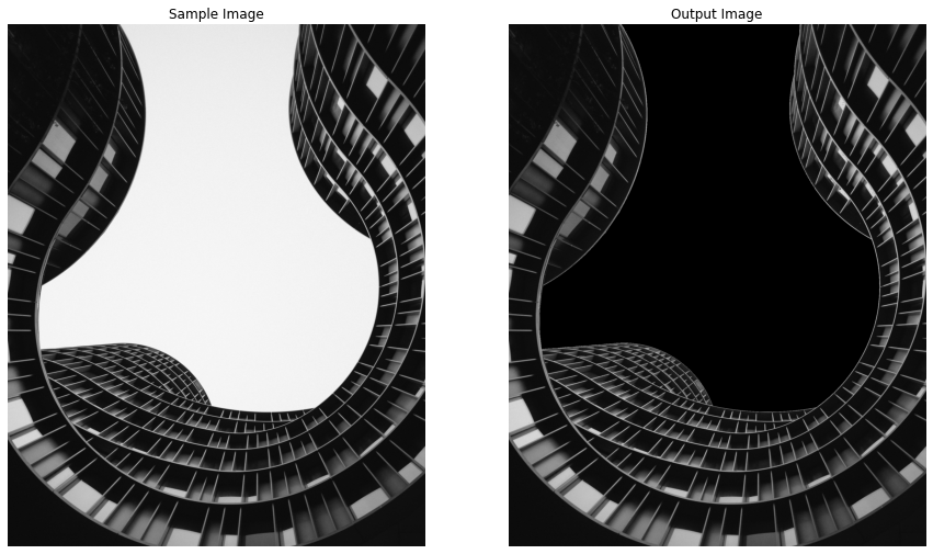
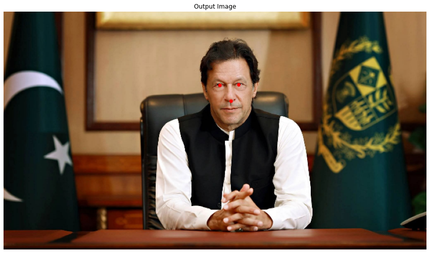
Almost all the image processing operations can be performed much more efficiently using these LookUp Tables like increasing/decreasing image brightness, saturation, contrast, even changing specific colors in images like the black and white color shift done in the image below.
Stunning! right? let’s try to perform this color shift on a few sample images. First, we will construct a LookUp Table mapping all the pixel values greater than 220 (white) to 0 (black) and then transform an image according to the lookup table using the cv2.LUT() function.
src: – It is the input array (image) of 8-bit elements.
lut: – It is the look-up table of 256 elements.
Returns:
dst: – It is the output array of the same size and number of channels as src, and the same depth as lut.
Note:In the case of a multi-channel input array (src), the table (lut) should either have a single channel (in this case the same table is used for all channels) or the same number of channels as in the input array (src).
# Read a sample image.
image = cv2.imread('media/sample.jpg')

# Initialize a list to store the lookuptable mapping.
white_to_black_table = []

# Iterate over 256 times.
# As images have pixels intensities [0-255].
for i in range(256):

    # Check if i is greater than 220.
    if i > 220:

        # Append 0 into the list.
        # This will convert pixels > 220 to 0.
        white_to_black_table.append(0)

    # Otherwise.
    else:

        # Append i into the list.
        # The pixels <= 220 will remain the same.
        white_to_black_table.append(i)

# Transform the image according to the lookup table.
output_image = cv2.LUT(image, np.array(white_to_black_table).astype("uint8"))

# Display the original sample image and the resultant image.
plt.figure(figsize=[15,15])
plt.subplot(121);plt.imshow(image[:,:,::-1]);plt.title("Sample Image");plt.axis('off');
plt.subplot(122);plt.imshow(output_image[:,:,::-1]);plt.title("Output Image");plt.axis('off');
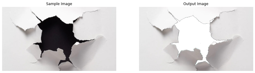
As you can see it worked as expected. Now let’s construct another LookUp Table mapping all the pixel values less than 50 (black) to 255 (white) and then transform another sample image to switch the black color in the image with white.
# Read another sample image.
image = cv2.imread('media/wall.jpg')

# Initialize a list to store the lookuptable mapping.
black_to_white_table = []

# Iterate over 256 times.
for i in range(256):

    # Check if i is less than 50.
    if i < 50:

        # Append 255 into the list.
        black_to_white_table.append(255)

    # Otherwise.
    else:

        # Append i into the list.
        black_to_white_table.append(i)

# Transform the image according to the lookup table.
output_image = cv2.LUT(image, np.array(black_to_white_table).astype("uint8"))

# Display the original sample image and the resultant image.
plt.figure(figsize=[15,15])
plt.subplot(121);plt.imshow(image[:,:,::-1]);plt.title("Sample Image");plt.axis('off');
plt.subplot(122);plt.imshow(output_image[:,:,::-1]);plt.title("Output Image");plt.axis('off');
The Black to white shift is also working perfectly fine. You can perform a similar shift with any color you want and this technique can be really helpful in efficiently changing green background screens from high-resolution videos and creating some interesting effects.
But we still don’t have an idea how much computational power and time these LookUp Tables save and are they worth trying? Well, this completely depends upon your use case, the number of images you want to transform, the resolution of the images you are working on, etc.
How about we perform a black to white shift on a few images with and without LookUp Tables and note the execution time to get an idea of the time difference? You can change the number of images and their resolution according to your use case.
# Set the number of images and their resolution.
num_of_images = 100
image_resolution = (960, 1280)
First, let’s do it without using LookUp Tables.
%%time
# Use magic command to measure execution time.

# Iterate over the number of times equal to the number of images.
for i in range(num_of_images):

    # Create a dummy image with each pixel value equal to 0.
    image = np.zeros(shape=image_resolution, dtype=np.uint8)

    # Convert pixels < 50 to 255.
    image[image<50] = 255
Wall time: 194 ms
We have the execution time without using LookUp Tables, now let’s check the difference by performing the same operation utilizing LookUp Tables. First we will create the look up Table, this only has to be done once.
# Initialize a list to store the lookuptable mapping.
table = []

# Iterate over 256 times.
for i in range(256):

     # Check if i is less than 50.
    if i < 50:

        # Append 255 into the list.
        table.append(255)

    # Otherwise.
    else:

        # Append i into the list.
        table.append(i)
Now we’ll use the look up table created above in action
%%time
# Use magic command to measure execution time.

# Iterate over the number of times equal to the number of images.
for i in range(num_of_images):

    # Create a dummy image with each pixel value equal to 0.
    image = np.zeros(shape=image_resolution, dtype=np.uint8)

    # Transform the image according to the lookup table.
    cv2.LUT(image, np.array(table).astype("uint8"))
Wall time: 81.2 ms
So the time taken in the second approach (LookUp Tables) is significantly lesser while the results are the same.
Applying Color Filters on Images/Videos
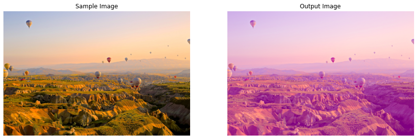
Finally comes the fun part, Color Filters that give interesting lighting effects to images, simply by modifying pixel values of different color channels (R,G,B) of images and we will create some of these effects utilizing LookUp tables.
We will first construct a lookup table, containing the mapping that we will need to apply different color filters.
# Initialize a list to store the lookuptable for the color filter.
color_table = []

# Iterate over 128 times from 128-255.
for i in range(128, 256):

    # Extend the table list and add the i two times in the list.
    # We want to increase pixel intensities that's why we are adding only values > 127.
    # We are adding same value two times because we need total 256 elements in the list.
    color_table.extend([i, i])
# We just added each element 2 times.
print(color_table[:10], "Length of table: " + str(len(color_table)))
Now we will create a function applyColorFilter() that will utilize the lookup table we created above, to increase pixel intensities of specified channels of images and videos and will display the resultant image along with the original image or return the resultant image depending upon the passed arguments.
def applyColorFilter(image, channels_indexes, display=True):
    '''
    This function will apply different interesting color lighting effects on an image.
    Args:
        image:            The image on which the color filter is to be applied.
        channels_indexes: A list of channels indexes that are required to be transformed.
        display:          A boolean value that is if set to true the function displays the original image,
                          and the output image with the color filter applied and returns nothing.
    Returns:
        output_image: The transformed resultant image on which the color filter is applied.
    '''

    # Access the lookuptable containing the mapping we need.
    global color_table

    # Create a copy of the image.
    output_image = image.copy()

    # Iterate over the indexes of the channels to modify.
    for channel_index in channels_indexes:

        # Transform the channel of the image according to the lookup table.
        output_image[:,:,channel_index] = cv2.LUT(output_image[:,:,channel_index],
                                                  np.array(color_table).astype("uint8"))

    # Check if the original input image and the resultant image are specified to be displayed.
    if display:

        # Display the original input image and the resultant image.
        plt.figure(figsize=[15,15])
        plt.subplot(121);plt.imshow(image[:,:,::-1]);plt.title("Sample Image");plt.axis('off');
        plt.subplot(122);plt.imshow(output_image[:,:,::-1]);plt.title("Output Image");plt.axis('off');

    # Otherwise
    else:

        # Return the resultant image.
        return output_image
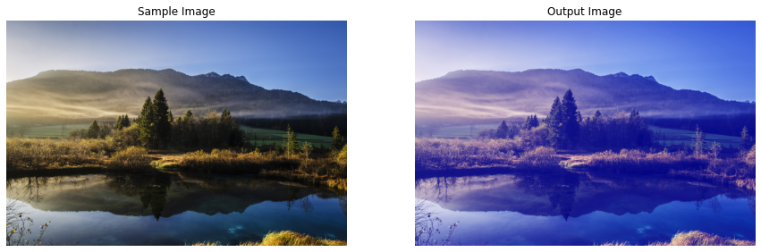
Now we will utilize the function applyColorFilter() to apply different color effects on a few sample images and display the results.
# Read a sample image and apply color filter on it.
image = cv2.imread('media/sample1.jpg')
applyColorFilter(image, channels_indexes=[0])
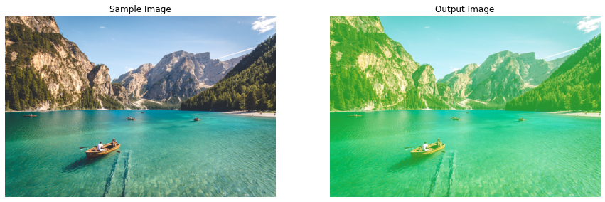
# Read another sample image and apply color filter on it.
image = cv2.imread('media/sample2.jpg')
applyColorFilter(image, channels_indexes=[1])
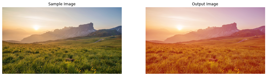
# Read another sample image and apply color filter on it.
image = cv2.imread('media/sample3.jpg')
applyColorFilter(image, channels_indexes=[2])
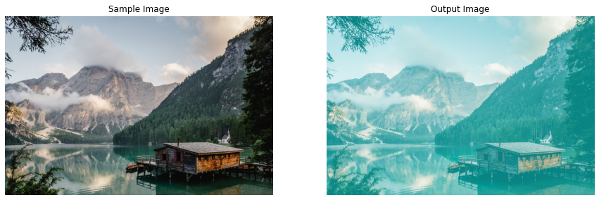
# Read another sample image and apply color filter on it.
image = cv2.imread('media/sample4.jpg')
applyColorFilter(image, channels_indexes=[0, 1])
# Read another sample image and apply color filter on it.
image = cv2.imread('media/sample5.jpg')
applyColorFilter(image, channels_indexes=[0, 2])
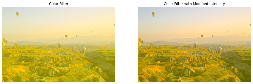
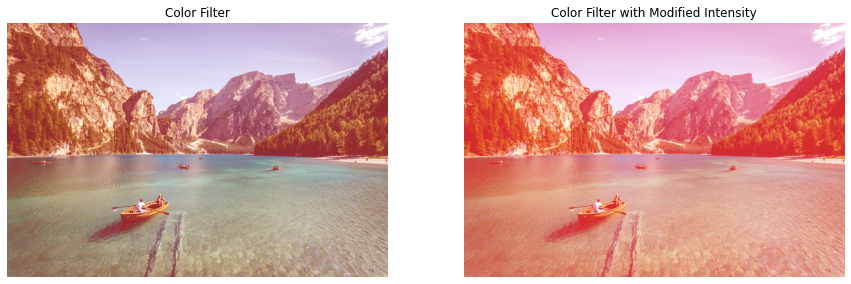
Cool! right? the results are astonishing but some of them are feeling a bit too much. So how about we will create another function changeIntensity() to control the intensity of these filters, again by utilizing LookUpTables. The function will simply increase or decrease the pixel intensities of the same color channels that were modified by the applyColorFilter() function and will display the results or return the resultant image depending upon the passed arguments.
For modifying the pixel intensities we will use the Gamma Correction technique, also known as the Power Law Transform. Its a nonlinear operation normally used to correct the brightness of an image using the following equation:
O=(I255)γ×255
Here γ<1 will increase the pixel intensities while γ>1 will decrease the pixel intensities and the filter effect. To perform the process, we will first construct a lookup table using the equation above.
# Initialize a variable to store previous gamma value.
prev_gamma = 1.0

# Initialize a list to store the lookuptable for the change intensity operation.
intensity_table = []

# Iterate over 256 times.
for i in range(256):

    # Calculate the mapping output value for the i input value,
    # and clip (limit) the values between 0 and 255.
    # Also append it into the look-up table list.
    intensity_table.append(np.clip(a=pow(i/255.0, prev_gamma)*255.0, a_min=0, a_max=255))
And then we will create the changeIntensity() function, which will use the table we have constructed and will re-construct the table every time the gamma value changes.
def changeIntensity(image, scale_factor, channels_indexes, display=True):
    '''
    This function will change intensity of the color filters.
    Args:
        image:            The image on which the color filter intensity is required to be changed.
        scale_factor:     A number that will be used to calculate the required gamma value.
        channels_indexes: A list of indexes of the channels on which the color filter was applied.
        display:          A boolean value that is if set to true the function displays the original image,
                          and the output image, and returns nothing.
    Returns:
        output_image: A copy of the input image with the color filter intensity changed.
    '''

    # Access the previous gamma value and the table contructed
    # with the previous gamma value.
    global prev_gamma, intensity_table

    # Create a copy of the input image.
    output_image = image.copy()

    # Calculate the gamma value from the passed scale factor.
    gamma = 1.0/scale_factor

    # Check if the previous gamma value is not equal to the current gamma value.
    if gamma != prev_gamma:

        # Update the intensity lookuptable to an empty list.
        # We will have to re-construct the table for the new gamma value.
        intensity_table = []

        # Iterate over 256 times.
        for i in range(256):

            # Calculate the mapping output value for the i input value
            # And clip (limit) the values between 0 and 255.
            # Also append it into the look-up table list.
            intensity_table.append(np.clip(a=pow(i/255.0, gamma)*255.0, a_min=0, a_max=255))

        # Update the previous gamma value.
        prev_gamma = gamma

    # Iterate over the indexes of the channels.
    for channel_index in channels_indexes:

        # Change intensity of the channel of the image according to the lookup table.
        output_image[:,:,channel_index] = cv2.LUT(output_image[:,:,channel_index],
                                                  np.array(intensity_table).astype("uint8"))

    # Check if the original input image and the output image are specified to be displayed.
    if display:

        # Display the original input image and the output image.
        plt.figure(figsize=[15,15])
        plt.subplot(121);plt.imshow(image[:,:,::-1]);plt.title("Color Filter");plt.axis('off');
        plt.subplot(122);plt.imshow(output_image[:,:,::-1]);plt.title("Color Filter with Modified Intensity")
        plt.axis('off')

    # Otherwise.
    else:

        # Return the output image.
        return output_image
Now let’s check how the changeIntensity() function works on a few sample images.
# Read a sample image and apply color filter on it with intensity 0.6.
image = cv2.imread('media/sample5.jpg')
image = applyColorFilter(image, channels_indexes=[1, 2], display=False)
changeIntensity(image, scale_factor=0.6, channels_indexes=[1, 2])
# Read another sample image and apply color filter on it with intensity 3.
image = cv2.imread('media/sample2.jpg')
image = applyColorFilter(image, channels_indexes=[2], display=False)
changeIntensity(image, scale_factor=3, channels_indexes=[2])
Apply Color Filters On Real-Time Web-cam Feed
The results on the images are exceptional, now let’s check how these filters will look on a real-time webcam feed. But first, we will create a mouse event callback function selectFilter(), that will allow us to select the filter to apply by clicking on the filter preview on the top of the frame in real-time.
def selectFilter(event, x, y, flags, userdata):
    '''
    This function will update the current filter applied on the frame based on different mouse events.
    Args:
        event:    The mouse event that is captured.
        x:        The x-coordinate of the mouse pointer position on the window.
        y:        The y-coordinate of the mouse pointer position on the window.
        flags:    It is one of the MouseEventFlags constants.
        userdata: The parameter passed from the `cv2.setMouseCallback()` function.
    '''

    # Access the filter applied and the channels indexes variable.
    global filter_applied, channels_indexes

    # Check if the left mouse button is pressed.
    if event == cv2.EVENT_LBUTTONDOWN:

        # Check if the mouse pointer y-coordinate is less than equal to a certain threshold.
        if y <= 10+preview_height:

            # Check if the mouse pointer x-coordinate is over the Blue filter ROI.
            if x > (int(frame_width//1.25)-preview_width//2) and \
            x < (int(frame_width//1.25)-preview_width//2)+preview_width:

                # Update the filter applied variable value to Blue.
                filter_applied = 'Blue'

                # Update the channels indexes list to store the
                # indexes of the channels to modify for the Blue filter.
                channels_indexes = [0]

            # Check if the mouse pointer x-coordinate is over the Green filter ROI.
            elif x>(int(frame_width//1.427)-preview_width//2) and \
            x<(int(frame_width//1.427)-preview_width//2)+preview_width:

                # Update the filter applied variable value to Green.
                filter_applied = 'Green'

                # Update the channels indexes list to store the
                # indexes of the channels to modify for the Green filter.
                channels_indexes = [1]

            # Check if the mouse pointer x-coordinate is over the Red filter ROI.
            elif x>(frame_width//1.665-preview_width//2) and \
            x<(frame_width//1.665-preview_width//2)+preview_width:

                # Update the filter applied variable value to Red.
                filter_applied = 'Red'

                # Update the channels indexes list to store the
                # indexes of the channels to modify for the Red filter.
                channels_indexes = [2]

            # Check if the mouse pointer x-coordinate is over the Normal frame ROI.
            elif x>(int(frame_width//2)-preview_width//2) and \
            x<(int(frame_width//2)-preview_width//2)+preview_width:

                # Update the filter applied variable value to Normal.
                filter_applied = 'Normal'

                # Update the channels indexes list to empty list.
                # As no channels are modified in the Normal filter.
                channels_indexes = []

            # Check if the mouse pointer x-coordinate is over the Cyan filter ROI.
            elif x>(int(frame_width//2.5)-preview_width//2) and \
            x<(int(frame_width//2.5)-preview_width//2)+preview_width:

                # Update the filter applied variable value to Cyan Filter.
                filter_applied = 'Cyan'

                # Update the channels indexes list to store the
                # indexes of the channels to modify for the Cyan filter.
                channels_indexes = [0, 1]

            # Check if the mouse pointer x-coordinate is over the Purple filter ROI.
            elif x>(int(frame_width//3.33)-preview_width//2) and \
            x<(int(frame_width//3.33)-preview_width//2)+preview_width:

                # Update the filter applied variable value to Purple.
                filter_applied = 'Purple'

                # Update the channels indexes list to store the
                # indexes of the channels to modify for the Purple filter.
                channels_indexes = [0, 2]

            # Check if the mouse pointer x-coordinate is over the Yellow filter ROI.
            elif x>(int(frame_width//4.99)-preview_width//2) and \
            x<(int(frame_width//4.99)-preview_width//2)+preview_width:

                # Update the filter applied variable value to Yellow.
                filter_applied = 'Yellow'

                # Update the channels indexes list to store the
                # indexes of the channels to modify for the Yellow filter.
                channels_indexes = [1, 2]
Now without further ado, let’s test the filters on a real-time webcam feed, we will be switching between the filters by utilizing the selectFilter() function created above and will use a trackbar to change the intensity of the filter applied in real-time.
# Initialize the VideoCapture object to read from the webcam.
camera_video = cv2.VideoCapture(0)
camera_video.set(3,1280)
camera_video.set(4,960)

# Create a named resizable window.
cv2.namedWindow('Color Filters', cv2.WINDOW_NORMAL)

# Create the function for the trackbar since its mandatory.
def nothing(x):
    pass

# Create trackbar named Intensity with the range [0-100].
cv2.createTrackbar('Intensity', 'Color Filters', 50, 100, nothing)

# Attach the mouse callback function to the window.
cv2.setMouseCallback('Color Filters', selectFilter)

# Initialize a variable to store the current applied filter.
filter_applied = 'Normal'

# Initialize a list to store the indexes of the channels
# that were modified to apply the current filter.
# This list will be required to change intensity of the applied filter.
channels_indexes = []

# Iterate until the webcam is accessed successfully.
while camera_video.isOpened():

    # Read a frame.
    ok, frame = camera_video.read()

    # Check if frame is not read properly then
    # continue to the next iteration to read the next frame.
    if not ok:
        continue

    # Flip the frame horizontally for natural (selfie-view) visualization.
    frame = cv2.flip(frame, 1)

    # Get the height and width of the frame of the webcam video.
    frame_height, frame_width, _ = frame.shape

    # Initialize a dictionary and store the copies of the frame with the
    # filters applied by transforming some different channels combinations.
    filters = {'Normal': frame.copy(),
               'Blue': applyColorFilter(frame, channels_indexes=[0], display=False),
               'Green': applyColorFilter(frame, channels_indexes=[1], display=False),
               'Red': applyColorFilter(frame, channels_indexes=[2], display=False),
               'Cyan': applyColorFilter(frame, channels_indexes=[0, 1], display=False),
               'Purple': applyColorFilter(frame, channels_indexes=[0, 2], display=False),
               'Yellow': applyColorFilter(frame, channels_indexes=[1, 2], display=False)}

    # Initialize a list to store the previews of the filters.
    filters_previews = []

    # Iterate over the filters dictionary.
    for filter_name, filter_applied_frame in filters.items():

        # Check if the filter we are iterating upon, is applied.
        if filter_applied == filter_name:

            # Set color to green.
            # This will be the border color of the filter preview.
            # And will be green for the filter applied and white for the other filters.
            color = (0,255,0)

        # Otherwise.
        else:

            # Set color to white.
            color = (255,255,255)

        # Make a border around the filter we are iterating upon.
        filter_preview = cv2.copyMakeBorder(src=filter_applied_frame, top=100,
                                            bottom=100, left=10, right=10,
                                            borderType=cv2.BORDER_CONSTANT, value=color)

        # Resize the filter applied frame to the 1/10th of its current width
        # while keeping the aspect ratio constant.
        filter_preview = cv2.resize(filter_preview,
                                    (frame_width//10,
                                     int(((frame_width//10)/frame_width)*frame_height)))

        # Append the filter preview into the list.
        filters_previews.append(filter_preview)

    # Update the frame with the currently applied Filter.
    frame = filters[filter_applied]

    # Get the value of the filter intensity from the trackbar.
    filter_intensity = cv2.getTrackbarPos('Intensity', 'Color Filters')/100 + 0.5

    # Check if the length of channels indexes list is > 0.
    if len(channels_indexes) > 0:

        # Change the intensity of the applied filter.
        frame = changeIntensity(frame, filter_intensity,
                                channels_indexes,  display=False)

    # Get the new height and width of the previews.
    preview_height, preview_width, _ = filters_previews[0].shape

    # Overlay the resized preview filter images over the frame by updating
    # its pixel values in the region of interest.
    #######################################################################################

    # Overlay the Blue Filter preview on the frame.
    frame[10: 10+preview_height,
          (int(frame_width//1.25)-preview_width//2):\
          (int(frame_width//1.25)-preview_width//2)+preview_width] = filters_previews[1]

    # Overlay the Green Filter preview on the frame.
    frame[10: 10+preview_height,
          (int(frame_width//1.427)-preview_width//2):\
          (int(frame_width//1.427)-preview_width//2)+preview_width] = filters_previews[2]

    # Overlay the Red Filter preview on the frame.
    frame[10: 10+preview_height,
          (int(frame_width//1.665)-preview_width//2):\
          (int(frame_width//1.665)-preview_width//2)+preview_width] = filters_previews[3]

    # Overlay the normal frame (no filter) preview on the frame.
    frame[10: 10+preview_height,
          (frame_width//2-preview_width//2):\
          (frame_width//2-preview_width//2)+preview_width] = filters_previews[0]

    # Overlay the Cyan Filter preview on the frame.
    frame[10: 10+preview_height,
          (int(frame_width//2.5)-preview_width//2):\
          (int(frame_width//2.5)-preview_width//2)+preview_width] = filters_previews[4]

    # Overlay the Purple Filter preview on the frame.
    frame[10: 10+preview_height,
      (int(frame_width//3.33)-preview_width//2):\
          (int(frame_width//3.33)-preview_width//2)+preview_width] = filters_previews[5]

    # Overlay the Yellow Filter preview on the frame.
    frame[10: 10+preview_height,
      (int(frame_width//4.99)-preview_width//2):\
          (int(frame_width//4.99)-preview_width//2)+preview_width] = filters_previews[6]

    #######################################################################################

    # Display the frame.
    cv2.imshow('Color Filters', frame)

    # Wait for 1ms. If a key is pressed, retreive the ASCII code of the key.
    k = cv2.waitKey(1) & 0xFF

    # Check if 'ESC' is pressed and break the loop.
    if(k == 27):
        break

# Release the VideoCapture Object and close the windows.
camera_video.release()
cv2.destroyAllWindows()
Output Video:
As expected, the results are fascinating on videos as well.
Assignment (Optional)
Apply a different color filter on the foreground and a different color filter on the background, and share the results with me in the comments section. You can use MediaPipe’s Selfie Segmentation solution to segment yourself in order to differentiate the foreground and the background.
Join My Course Computer Vision For Building Cutting Edge Applications Course
The only course out there that goes beyond basic AI Applications and teaches you how to create next-level apps that utilize physics, deep learning, classical image processing, hand and body gestures. Don’t miss your chance to level up and take your career to new heights
You’ll Learn about:
Creating GUI interfaces for python AI scripts.
Creating .exe DL applications
Using a Physics library in Python & integrating it with AI
Advance Image Processing Skills
Advance Gesture Recognition with Mediapipe
Task Automation with AI & CV
Training an SVM machine Learning Model.
Creating & Cleaning an ML dataset from scratch.
Training DL models & how to use CNN’s & LSTMS.
Creating 10 Advance AI/CV Applications
& More
Whether you’re a seasoned AI professional or someone just looking to start out in AI, this is the course that will teach you, how to Architect & Build complex, real world and thrilling AI applications
Today, in this tutorial, we went over every bit of detail about the LookUp Tables, we learned what these LookUp Tables are, why they are useful and the use cases in which you should prefer them. Then we used these LookUp Tables to create different lighting effects (called Color Filters) on images and videos.
We utilized the concepts we learned about the Mouse Events and TrackBars in the previous tutorial of the series to switch between filters from the available options and change the applied filter intensity in real-time. Now in the next and final tutorial of the series, we will create some famous Instagram filters, so stick around for that.
And keep in mind that our intention was to teach you these crucial image processing concepts so that’s why we went for building the whole application using OpenCV (to keep the tutorial simple) but I do not think we have done justice with the user interface part, there’s room for a ton of improvements.
There are a lot of GUI libraries like PyQt, Pygame, and Kivi (to name a few) that you can use in order to make the UI more appealing for this application.
In the previous tutorial of this series, we had covered Look Up Tables in-depth and utilized them to create some interesting lighting effects on images/videos. Now in this one, we are gonna level up the game by creating 10 very interesting and cool Instagram filters.
The Filters which are gonna be covered are; Warm Filter, Cold Filter, Gotham Filter, GrayScale Filter, Sepia Filter, Pencil Sketch Filter, Sharpening Filter, Detail Enhancing Filter, Invert Filter, and Stylization Filter.
You must have used at least one of these and maybe have wondered how these are created, what’s the magic (math) behind these. We are gonna cover all this in-depth in today’s tutorial and you will learn a ton of cool image transformation techniques with OpenCV so buckle up and keep reading the tutorial.
This is the last tutorial of our 3 part Creating Instagram Filters series. All three posts are titled as:
Part 3: Designing Advanced Image Filters in OpenCV (Current tutorial)
3-4 Filters in this tutorial use Look Up Tables (LUT) which were explained in the previous tutorial, so make sure to go over that one if you haven’t already. Also, we have used mouse events to switch between filters in real-time and had covered mouse events in the first post of the series, so go over that tutorial as well if you don’t know how to use mouse events in OpenCV.
The tutorial is pretty simple and straightforward, but for a detailed explanation you can check out the YouTube video above, although this blog post alone does have enough details to help you follow along.
We will start by importing the required libraries.
import cv2
import pygame
import numpy as np
import matplotlib.pyplot as plt
from scipy.interpolate import UnivariateSpline
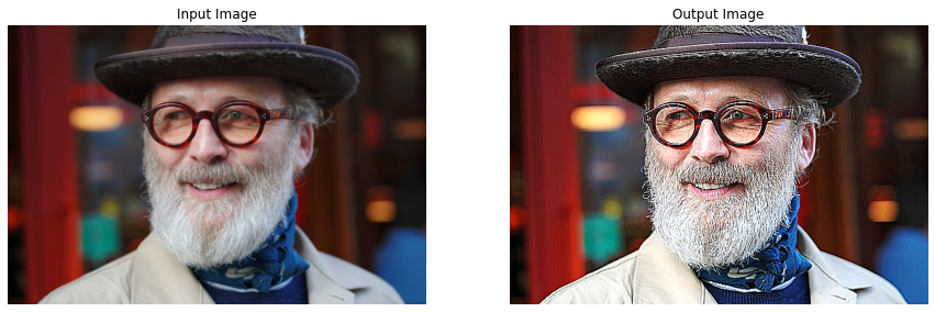
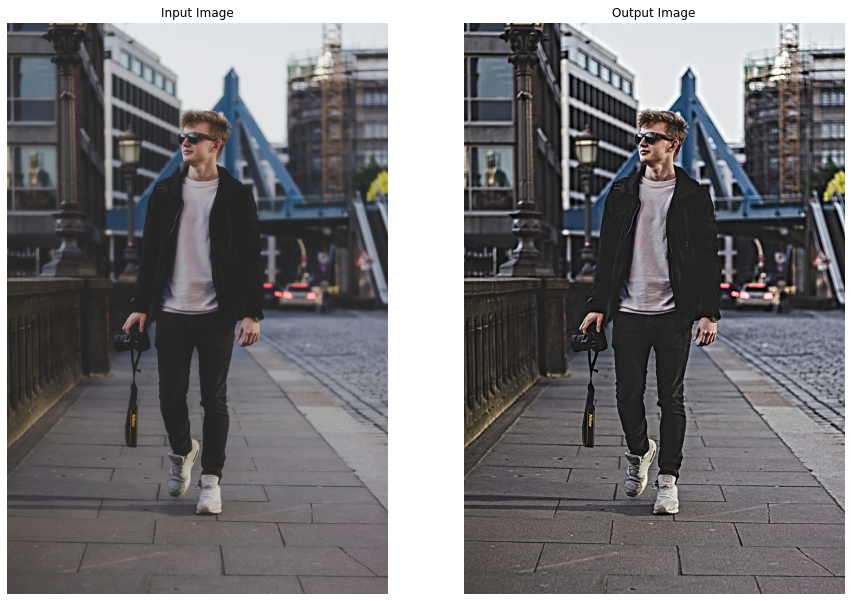
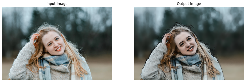
Creating Warm Filter-like Effect
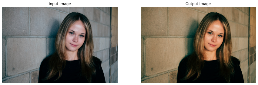
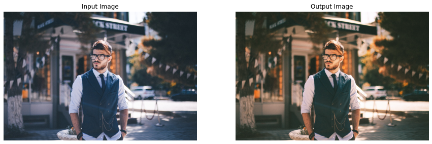
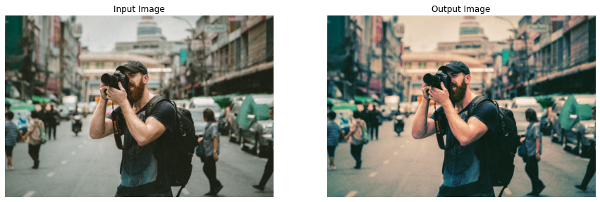
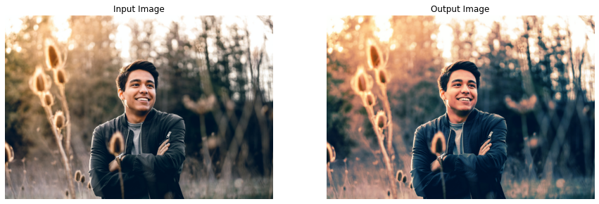
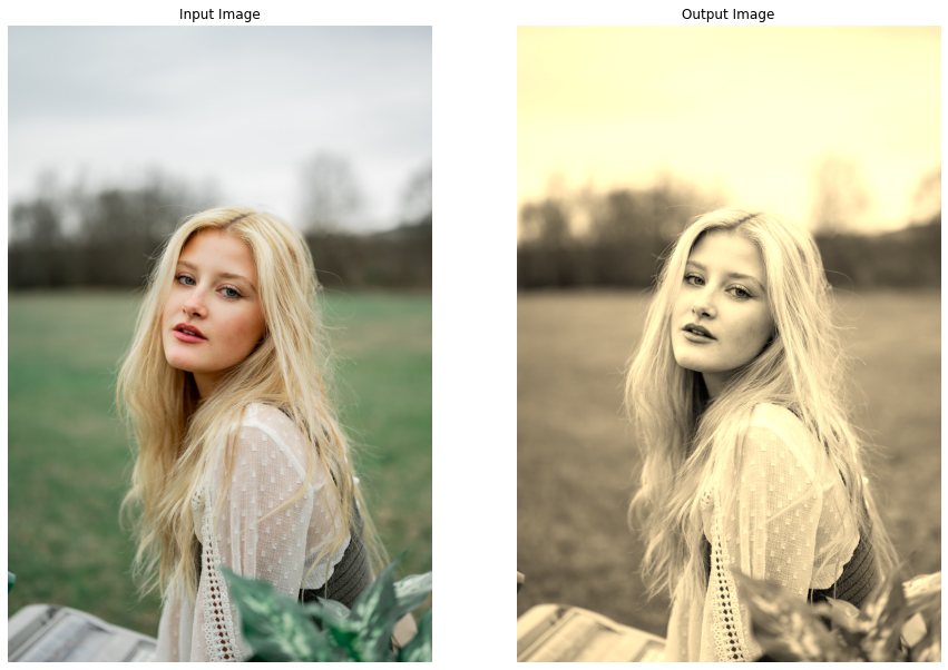
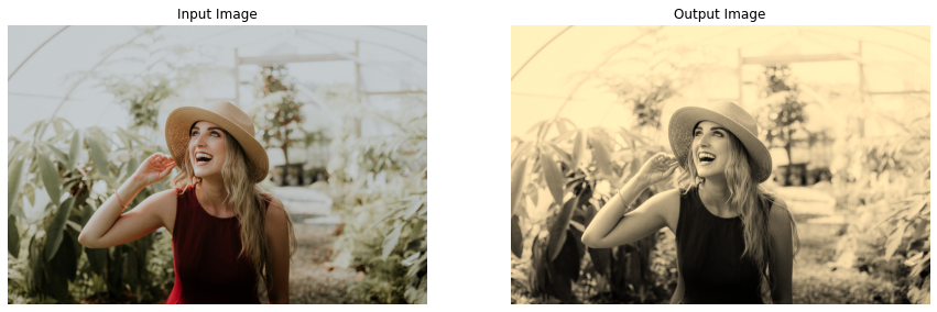
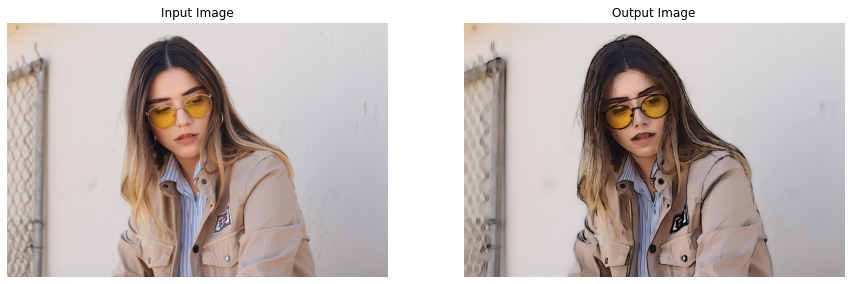
The first filter is gonna be the famous Warm Effect, it absorbs blue cast in images, often caused by electronic flash or outdoor shade, and improves skin tones. This gives a kind of warm look to images that’s why it is called the Warm Effect. To apply this to images and videos, we will create a function applyWarm() that will decrease the pixel intensities of the blue channel and increase the intensities of the red channel of an image/frame by utilizing Look Up tables ( that we learned about in the previous tutorial).
So first, we will have to construct the Look Up Tables required to increase/decrease pixel intensities. For this purpose, we will be using the scipy.interpolate.UnivariateSpline() function to get the required input-output mapping.
# Construct a lookuptable for increasing pixel values.
# We are giving y values for a set of x values.
# And calculating y for [0-255] x values accordingly to the given range.
increase_table = UnivariateSpline(x=[0, 64, 128, 255], y=[0, 75, 155, 255])(range(256))

# Similarly construct a lookuptable for decreasing pixel values.
decrease_table = UnivariateSpline(x=[0, 64, 128, 255], y=[0, 45, 95, 255])(range(256))

# Display the first 10 mappings from the constructed tables.
print(f'First 10 elements from the increase table: \n {increase_table[:10]}\n')
print(f'First 10 elements from the decrease table:: \n {decrease_table[:10]}')
Output:
First 10 elements from the increase table: [7.32204295e-15 1.03827895e+00 2.08227359e+00 3.13191257e+00 4.18712454e+00 5.24783816e+00 6.31398207e+00 7.38548493e+00 8.46227539e+00 9.54428209e+00]
First 10 elements from the decrease table:: [-5.69492230e-15 7.24142824e-01 1.44669675e+00 2.16770636e+00 2.88721627e+00 3.60527107e+00 4.32191535e+00 5.03719372e+00 5.75115076e+00 6.46383109e+00]
Now that we have the Look Up Tables we need, we can move on to transforming the red and blue channel of the image/frame using the function cv2.LUT(). And to split and merge the channels of the image/frame, we will be using the function cv2.split() and cv2.merge() respectively. The applyWarm() function (like every other function in this tutorial) will display the resultant image along with the original image or return the resultant image depending upon the passed arguments.
def applyWarm(image, display=True):
    '''
    This function will create instagram Warm filter like effect on an image.
    Args:
        image:  The image on which the filter is to be applied.
        display: A boolean value that is if set to true the function displays the original image,
                 and the output image, and returns nothing.
    Returns:
        output_image: A copy of the input image with the Warm filter applied.
    '''

    # Split the blue, green, and red channel of the image.
    blue_channel, green_channel, red_channel  = cv2.split(image)

    # Increase red channel intensity using the constructed lookuptable.
    red_channel = cv2.LUT(red_channel, increase_table).astype(np.uint8)

    # Decrease blue channel intensity using the constructed lookuptable.
    blue_channel = cv2.LUT(blue_channel, decrease_table).astype(np.uint8)

    # Merge the blue, green, and red channel.
    output_image = cv2.merge((blue_channel, green_channel, red_channel))

    # Check if the original input image and the output image are specified to be displayed.
    if display:

        # Display the original input image and the output image.
        plt.figure(figsize=[15,15])
        plt.subplot(121);plt.imshow(image[:,:,::-1]);plt.title("Input Image");plt.axis('off');
        plt.subplot(122);plt.imshow(output_image[:,:,::-1]);plt.title("Output Image");plt.axis('off');

    # Otherwise.
    else:

        # Return the output image.
        return output_image
Now, let’s utilize the applyWarm() function created above to apply this warm filter on a few sample images.
# Read a sample image and apply Warm filter on it.
image = cv2.imread('media/sample1.jpg')
applyWarm(image)
# Read another sample image and apply Warm filter on it.
image = cv2.imread('media/sample2.jpg')
applyWarm(image)
Woah! Got the same results as the Instagram warm filter, with just a few lines of code. Now let’s move on to the next one.
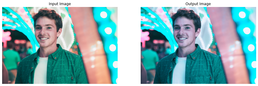
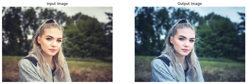
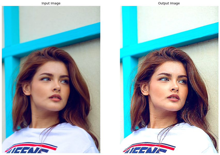
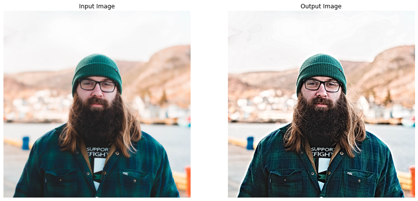
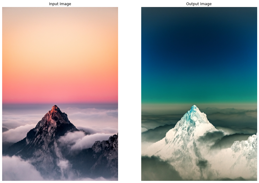
Creating Cold Filter-like Effect
This one is kind of the opposite of the above filter, it gives coldness look to images/videos by increasing the blue cast. To create this filter effect, we will define a function applyCold() that will increase the pixel intensities of the blue channel and decrease the intensities of the red channel of an image/frame by utilizing the same LookUp tables, we had constructed above.
For this one too, we will be using the cv2.split(), cv2.LUT() and cv2.merge() functions to split, transform, and merge the channels.
def applyCold(image, display=True):
    '''
    This function will create instagram Cold filter like effect on an image.
    Args:
        image:  The image on which the filter is to be applied.
        display: A boolean value that is if set to true the function displays the original image,
                 and the output image, and returns nothing.
    Returns:
        output_image: A copy of the input image with the Cold filter applied.
    '''

    # Split the blue, green, and red channel of the image.
    blue_channel, green_channel, red_channel = cv2.split(image)

    # Decrease red channel intensity using the constructed lookuptable.
    red_channel = cv2.LUT(red_channel, decrease_table).astype(np.uint8)

    # Increase blue channel intensity using the constructed lookuptable.
    blue_channel = cv2.LUT(blue_channel, increase_table).astype(np.uint8)

    # Merge the blue, green, and red channel.
    output_image = cv2.merge((blue_channel, green_channel, red_channel))

    # Check if the original input image and the output image are specified to be displayed.
    if display:

        # Display the original input image and the output image.
        plt.figure(figsize=[15,15])
        plt.subplot(121);plt.imshow(image[:,:,::-1]);plt.title("Input Image");plt.axis('off');
        plt.subplot(122);plt.imshow(output_image[:,:,::-1]);plt.title("Output Image");plt.axis('off');

    # Otherwise.
    else:

        # Return the output image.
        return output_image
Now we will test this cold filter effect utilizing the applyCold() function on some sample images.
# Read a sample image and apply cold filter on it.
image = cv2.imread('media/sample3.jpg')
applyCold(image)
# Read another sample image and apply cold filter on it.
image = cv2.imread('media/sample4.jpg')
applyCold(image)
Now we’ll use the look up table creat
Nice! Got the expected results for this one too.
Creating Gotham Filter-like Effect
Now the famous Gotham Filter comes in, you must have heard or used this one on Instagram, it gives a warm reddish type look to images. We will try to apply a similar effect to images and videos by creating a function applyGotham(), that will utilize LookUp tables to manipulate image/frame channels in the following manner.
Increase mid-tone contrast of the red channel
Boost the lower-mid values of the blue channel
Decrease the upper-mid values of the blue channel
But again first, we will have to construct the Look Up Tables required to perform the manipulation on the red and blue channels of the image. We will again utilize the scipy.interpolate.UnivariateSpline() function to get the required mapping.
# Construct a lookuptable for increasing midtone contrast.
# Meaning this table will decrease the difference between the midtone values.
# Again we are giving Ys for some Xs and calculating for the remaining ones ([0-255] by using range(256)).
midtone_contrast_increase = UnivariateSpline(x=[0, 25, 51, 76, 102, 128, 153, 178, 204, 229, 255],
                                             y=[0, 13, 25, 51, 76, 128, 178, 204, 229, 242, 255])(range(256))

# Construct a lookuptable for increasing lowermid pixel values.
lowermids_increase = UnivariateSpline(x=[0, 16, 32, 48, 64, 80, 96, 111, 128, 143, 159, 175, 191, 207, 223, 239, 255],
                                      y=[0, 18, 35, 64, 81, 99, 107, 112, 121, 143, 159, 175, 191, 207, 223, 239, 255])(range(256))

# Construct a lookuptable for decreasing uppermid pixel values.
uppermids_decrease = UnivariateSpline(x=[0, 16, 32, 48, 64, 80, 96, 111, 128, 143, 159, 175, 191, 207, 223, 239, 255],
                                      y=[0, 16, 32, 48, 64, 80, 96, 111, 128, 140, 148, 160, 171, 187, 216, 236, 255])(range(256))

# Display the first 10 mappings from the constructed tables.
print(f'First 10 elements from the midtone contrast increase table: \n {midtone_contrast_increase[:10]}\n')
print(f'First 10 elements from the lowermids increase table: \n {lowermids_increase[:10]}\n')
print(f'First 10 elements from the uppermids decrease table:: \n {uppermids_decrease[:10]}')
First 10 elements from the midtone contrast increase table: [0.09416024 0.75724879 1.39938782 2.02149343 2.62448172 3.20926878 3.77677071 4.32790362 4.8635836 5.38472674]
First 10 elements from the lowermids increase table: [0.15030475 1.31080448 2.44957754 3.56865611 4.67007234 5.75585842 6.82804653 7.88866883 8.9397575 9.98334471]
First 10 elements from the uppermids decrease table:: [-0.27440589 0.8349419 1.93606131 3.02916902 4.11448171 5.19221607 6.26258878 7.32581654 8.38211602 9.4317039 ]
Now that we have the required mappings, we can move on to creating the function applyGotham() that will utilize these LookUp tables to apply the required effect.
def applyGotham(image, display=True):
    '''
    This function will create instagram Gotham filter like effect on an image.
    Args:
        image:   The image on which the filter is to be applied.
        display: A boolean value that is if set to true the function displays the original image,
                 and the output image, and returns nothing.
    Returns:
        output_image: A copy of the input image with the Gotham filter applied.
    '''

    # Split the blue, green, and red channel of the image.
    blue_channel, green_channel, red_channel = cv2.split(image)

    # Boost the mid-tone red channel contrast using the constructed lookuptable.
    red_channel = cv2.LUT(red_channel, midtone_contrast_increase).astype(np.uint8)

    # Boost the Blue channel in lower-mids using the constructed lookuptable.
    blue_channel = cv2.LUT(blue_channel, lowermids_increase).astype(np.uint8)

    # Decrease the Blue channel in upper-mids using the constructed lookuptable.
    blue_channel = cv2.LUT(blue_channel, uppermids_decrease).astype(np.uint8)

    # Merge the blue, green, and red channel.
    output_image = cv2.merge((blue_channel, green_channel, red_channel))

    # Check if the original input image and the output image are specified to be displayed.
    if display:

        # Display the original input image and the output image.
        plt.figure(figsize=[15,15])
        plt.subplot(121);plt.imshow(image[:,:,::-1]);plt.title("Input Image");plt.axis('off');
        plt.subplot(122);plt.imshow(output_image[:,:,::-1]);plt.title("Output Image");plt.axis('off');

    # Otherwise.
    else:

        # Return the output image.
        return output_image
Now, let’s test this Gotham effect utilizing the applyGotham() function on a few sample images and visualize the results.
# Read a sample image and apply Gotham filter on it.
image = cv2.imread('media/sample5.jpg')
applyGotham(image)
# Read another sample image and apply Gotham filter on it.
image = cv2.imread('media/sample6.jpg')
applyGotham(image)
Now w
Stunning results! Now, let’s move to a simple one.
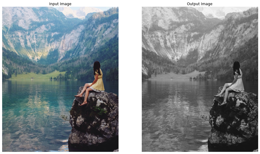
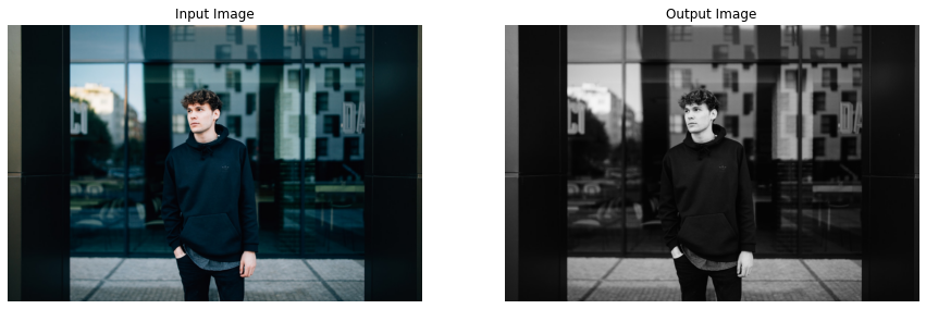
Creating Grayscale Filter-like Effect
Instagram also has a Grayscale filter also known as 50s TV Effect, it simply converts a (RGB) color image into a Grayscale (black and white) image. We can easily create a similar effect in OpenCV by using the cv2.cvtColor() function. So let’s create a function applyGrayscale() that will utilize cv2.cvtColor() function to apply this Grayscale filter-like effect on images and videos.
def applyGrayscale(image, display=True):
    '''
    This function will create instagram Grayscale filter like effect on an image.
    Args:
        image:  The image on which the filter is to be applied.
        display: A boolean value that is if set to true the function displays the original image,
                 and the output image, and returns nothing.
    Returns:
        output_image: A copy of the input image with the Grayscale filter applied.
    '''

    # Convert the image into the grayscale.
    gray = cv2.cvtColor(image, cv2.COLOR_BGR2GRAY)

    # Merge the grayscale (one-channel) image three times to make it a three-channel image.
    output_image = cv2.merge((gray, gray, gray))

    # Check if the original input image and the output image are specified to be displayed.
    if display:

        # Display the original input image and the output image.
        plt.figure(figsize=[15,15])
        plt.subplot(121);plt.imshow(image[:,:,::-1]);plt.title("Input Image");plt.axis('off');
        plt.subplot(122);plt.imshow(output_image[:,:,::-1]);plt.title("Output Image");plt.axis('off');

    # Otherwise.
    else:

        # Return the output image.
        return output_image
Now let’s utilize this applyGrayscale() function to apply the grayscale effect on a few sample images and display the results.
# Read a sample image| and apply Grayscale filter on it.
image = cv2.imread('media/sample7.jpg')
applyGrayscale(image)
# Read another sample image and apply Grayscale filter on it.
image = cv2.imread('media/sample8.jpg')
applyGrayscale(image)
Cool! Working as expected. Let’s move on to the next one.
Creating Sepia Filter-like Effect
I think this one is the most famous among all the filters we are creating today. This gives a warm reddish-brown vintage effect to images which makes the images look a bit ancient which is really cool. To apply this effect, we will create a function applySepia() that will utilize the cv2.transform() function and the fixed sepia matrix (standardized to create this effect, that you can easily find online) to serve the purpose.
def applySepia(image, display=True):
    '''
    This function will create instagram Sepia filter like effect on an image.
    Args:
        image:  The image on which the filter is to be applied.
        display: A boolean value that is if set to true the function displays the original image,
                 and the output image, and returns nothing.
    Returns:
        output_image: A copy of the input image with the Sepia filter applied.
    '''

    # Convert the image into float type to prevent loss during operations.
    image_float = np.array(image, dtype=np.float64)


    # Manually transform the image to get the idea of exactly whats happening.
    ##################################################################################################

    # Split the blue, green, and red channel of the image.
    blue_channel, green_channel, red_channel = cv2.split(image_float)

    # Apply the Sepia filter by perform the matrix multiplication between
    # the image and the sepia matrix.
    output_blue = (red_channel * .272) + (green_channel *.534) + (blue_channel * .131)
    output_green = (red_channel * .349) + (green_channel *.686) + (blue_channel * .168)
    output_red = (red_channel * .393) + (green_channel *.769) + (blue_channel * .189)

    # Merge the blue, green, and red channel.
    output_image = cv2.merge((output_blue, output_green, output_red))

    ##################################################################################################


        # OR Either create this effect by using OpenCV matrix transformation function.
    ##################################################################################################

    # Get the sepia matrix for BGR colorspace images.
    sepia_matrix = np.matrix([[.272, .534, .131],
                              [.349, .686, .168],
                              [.393, .769, .189]])

    # Apply the Sepia filter by perform the matrix multiplication between
    # the image and the sepia matrix.
    #output_image = cv2.transform(src=image_float, m=sepia_matrix)

    ##################################################################################################


    # Set the values > 255 to 255.
    output_image[output_image > 255] = 255

    # Convert the image back to uint8 type.
    output_image =  np.array(output_image, dtype=np.uint8)

    # Check if the original input image and the output image are specified to be displayed.
    if display:

        # Display the original input image and the output image.
        plt.figure(figsize=[15,15])
        plt.subplot(121);plt.imshow(image[:,:,::-1]);plt.title("Input Image");plt.axis('off');
        plt.subplot(122);plt.imshow(output_image[:,:,::-1]);plt.title("Output Image");plt.axis('off');

    # Otherwise.
    else:

        # Return the output image.
        return output_image
Now let’s check this sepia effect by utilizing the applySepia() function on a few sample images.
# Read a sample image and apply Sepia filter on it.
image = cv2.imread('media/sample9.jpg')
applySepia(image)
# Read another sample image and apply Sepia filter on it.
image = cv2.imread('media/sample18.jpg')
applySepia(image)
Spectacular results! Reminds me of the movies, I used to watch in my childhood ( Yes, I am that old 😜 ).
Creating Pencil Sketch Filter-like Effect
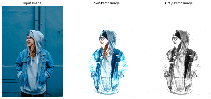
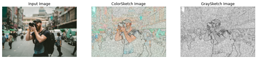
The next one is the Pencil Sketch Filter, creating a Pencil Sketch manually requires hours of hard work but luckily in OpenCV, we can do this in just one line of code by using the function cv2.pencilSketch() that give a pencil sketch-like effect to images. So lets create a function applyPencilSketch() to convert images/videos into Pencil Sketches utilizing the cv2.pencilSketch() function.
We will use the following funciton to applythe pencil sketch filter, this function retruns a grayscale sketch and a colored sketch of the image
This filter is a type of edge preserving filter, these filters have 2 Objectives, one is to give more weightage to pixels closer so that the blurring can be meaningfull and second to average only the similar intensity valued pixels to avoid the edges, so in this both of these objectives are controled by the two following parameters.
sigma_s Just like sigma in other smoothing filters this sigma value controls the area of the neighbourhood (Has Range between 0-200)
sigma_r This param controls the how dissimilar colors within the neighborhood will be averaged. For example a larger value will restrcit color variation and it will enforce that constant color stays throughout. (Has Range between 0-1)
shade_factor This has range 0-0.1 and controls how bright the final output will be by scaling the intensity.
def applyPencilSketch(image, display=True):
    '''
    This function will create instagram Pencil Sketch filter like effect on an image.
    Args:
        image:  The image on which the filter is to be applied.
        display: A boolean value that is if set to true the function displays the original image,
                 and the output image, and returns nothing.
    Returns:
        output_image: A copy of the input image with the Pencil Sketch filter applied.
    '''

    # Apply Pencil Sketch effect on the image.
    gray_sketch, color_sketch = cv2.pencilSketch(image, sigma_s=20, sigma_r=0.5, shade_factor=0.02)

    # Check if the original input image and the output image are specified to be displayed.
    if display:

        # Display the original input image and the output image.
        plt.figure(figsize=[15,15])
        plt.subplot(131);plt.imshow(image[:,:,::-1]);plt.title("Input Image");plt.axis('off');
        plt.subplot(132);plt.imshow(color_sketch[:,:,::-1]);plt.title("ColorSketch Image");plt.axis('off');
        plt.subplot(133);plt.imshow(gray_sketch, cmap='gray');plt.title("GraySketch Image");plt.axis('off');

    # Otherwise.
    else:

        # Return the output image.
        return color_sketch
Now we will apply this pencil sketch effect by utilizing the applyPencilSketch() function on a few sample images and visualize the results.
# Read a sample image and apply PencilSketch filter on it.
image = cv2.imread('media/sample11.jpg')
applyPencilSketch(image)
Now let’s check how the changeIntensity() functi
# Read another sample image and apply PencilSketch filter on it.
image = cv2.imread('media/sample5.jpg')
applyPencilSketch(image)
Amazing right? we created this effect with just a single line of code. So now, instead of spending hours manually sketching someone or something, you can take an image and apply this effect on it to get the results in seconds. And you can further tune the parameters of the cv2.pencilSketch() function to get even better results.
Creating Sharpening Filter-like Effect
Now let’s try to create the Sharpening Effect, this enhances the clearness of an image/video and decreases the blurriness which gives a new interesting look to the image/video. For this we will create a function applySharpening() that will utilize the cv2.filter2D() function to give the required effect to an image/frame passed to it.
 def applySharpening(image, display=True):
    '''
    This function will create the Sharpening filter like effect on an image.
    Args:
        image:  The image on which the filter is to be applied.
        display: A boolean value that is if set to true the function displays the original image,
                 and the output image, and returns nothing.
    Returns:
        output_image: A copy of the input image with the Sharpening filter applied.
    '''

    # Get the kernel required for the sharpening effect.
    sharpening_kernel = np.array([[-1, -1, -1],
                                  [-1, 9.2, -1],
                                  [-1, -1, -1]])

    # Apply the sharpening filter on the image.
    output_image = cv2.filter2D(src=image, ddepth=-1,
                                kernel=sharpening_kernel)

    # Check if the original input image and the output image are specified to be displayed.
    if display:

        # Display the original input image and the output image.
        plt.figure(figsize=[15,15])
        plt.subplot(121);plt.imshow(image[:,:,::-1]);plt.title("Input Image");plt.axis('off');
        plt.subplot(122);plt.imshow(output_image[:,:,::-1]);plt.title("Output Image");plt.axis('off');

    # Otherwise.
    else:

        # Return the output image.
        return output_image
Now, let’s see this in action utilizing the applySharpening() function created above on a few sample images.
# Read a sample image and apply Sharpening filter on it.
image = cv2.imread('media/sample12.jpg')
applySharpening(image)
# Read another sample image and apply Sharpening filter on it.
image = cv2.imread('media/sample13.jpg')
applySharpening(image)
Nice! this filter makes the original images look as if they are out of focus (blur).
Creating a Detail Enhancing Filter
Now this Filter is another type of edge preserving fitler and has the same parameters as the pencil sketch filter.This filter intensifies the details in images/videos, we’ll be using the function called cv2.detailEnhance(). let’s start by creating the a wrapper function applyDetailEnhancing(), that will utilize the cv2.detailEnhance() function to apply the needed effect.
def applyDetailEnhancing(image, display=True):
    '''
    This function will create the HDR filter like effect on an image.
    Args:
        image:  The image on which the filter is to be applied.
        display: A boolean value that is if set to true the function displays the original image,
                 and the output image, and returns nothing.
    Returns:
        output_image: A copy of the input image with the HDR filter applied.
    '''

    # Apply the detail enhancing effect by enhancing the details of the image.
    output_image = cv2.detailEnhance(image, sigma_s=15, sigma_r=0.15)

    # Check if the original input image and the output image are specified to be displayed.
    if display:

        # Display the original input image and the output image.
        plt.figure(figsize=[15,15])
        plt.subplot(121);plt.imshow(image[:,:,::-1]);plt.title("Input Image");plt.axis('off');
        plt.subplot(122);plt.imshow(output_image[:,:,::-1]);plt.title("Output Image");plt.axis('off');

    # Otherwise.
    else:

        # Return the output image.
        return output_image
Now, let’s test the function applyDetailEnhancing() created above on a few sample images.
# Read a sample image and apply Detail Enhancing filter on it.
image = cv2.imread('media/sample14.jpg')
applyDetailEnhancing(image)
# Read another sample image and apply Detail Enhancing filter on it.
image = cv2.imread('media/sample15.jpg')
applyDetailEnhancing(image)
Satisfying results! let’s move on to the next one.
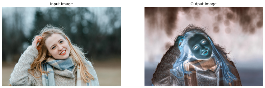
Creating Invert Filter-like Effect
This filter inverts the colors in images/videos meaning changes darkish colors into light and vice versa, which gives a very interesting look to images/videos. This can be accomplished using multiple approaches we can either utilize a LookUp table to perform the required transformation or subtract the image by 255 and take absolute of the results or just simply use the OpenCV function cv2.bitwise_not(). Let’s create a function applyInvert() to serve the purpose.
def applyInvert(image, display=True):
    '''
    This function will create the Invert filter like effect on an image.
    Args:
        image:  The image on which the filter is to be applied.
        display: A boolean value that is if set to true the function displays the original image,
                 and the output image, and returns nothing.
    Returns:
        output_image: A copy of the input image with the Invert filter applied.
    '''

    # Apply the Invert Filter on the image.
    output_image = cv2.bitwise_not(image)

    # Check if the original input image and the output image are specified to be displayed.
    if display:

        # Display the original input image and the output image.
        plt.figure(figsize=[15,15])
        plt.subplot(121);plt.imshow(image[:,:,::-1]);plt.title("Input Image");plt.axis('off');
        plt.subplot(122);plt.imshow(output_image[:,:,::-1]);plt.title("Output Image");plt.axis('off');

    # Otherwise.
    else:

        # Return the output image.
        return output_image
Let’s check this effect on a few sample images utilizing the applyInvert() function.
# Read a sample image and apply invert filter on it.
image = cv2.imread('media/sample16.jpg')
applyInvert(image)
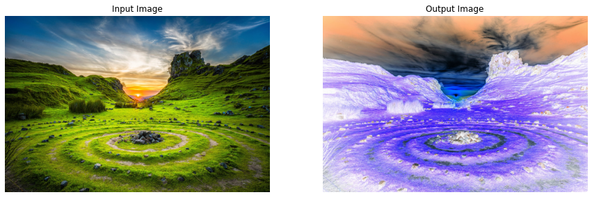
Looks a little scary, lets’s try it on a few landscape images.
# Read a landscape image and apply invert filter on it.
image = cv2.imread('media/sample19.jpg')
applyInvert(image)
# Read another landscape image and apply invert filter on it.
image = cv2.imread('media/sample20.jpg')
applyInvert(image)
Interesting effect! but I will definitely not recommend using this one on your own images, except if your intention is to scare someone xD.
Creating Stylization Filter-like Effect
Now let’s move on to the final one, which gives a painting-like effect to images. We will create a function applyStylization() that will utilize the cv2.stylization() function to apply this effect on images and videos. This one too will only need a single line of code.
def applyStylization(image, display=True):
    '''
    This function will create instagram cartoon-paint filter like effect on an image.
    Args:
        image:  The image on which the filter is to be applied.
        display: A boolean value that is if set to true the function displays the original image,
                 and the output image, and returns nothing.
    Returns:
        output_image: A copy of the input image with the cartoon-paint filter applied.
    '''

    # Apply stylization effect on the image.
    output_image = cv2.stylization(image, sigma_s=15, sigma_r=0.55)

    # Check if the original input image and the output image are specified to be displayed.
    if display:

        # Display the original input image and the output image.
        plt.figure(figsize=[15,15])
        plt.subplot(121);plt.imshow(image[:,:,::-1]);plt.title("Input Image");plt.axis('off');
        plt.subplot(122);plt.imshow(output_image[:,:,::-1]);plt.title("Output Image");plt.axis('off');

    # Otherwise.
    else:

        # Return the output image.
        return output_image
Now, as done for every other filter, we will utilize the function applyStylization() to test this effect on a few sample images.
# Read a sample image and apply Stylization filter on it.
image = cv2.imread('media/sample16.jpg')
applyStylization(image)
# Read another sample image and apply Stylization filter on it.
image = cv2.imread('media/sample17.jpg')
applyStylization(image)
Again got fascinating results! Wasn’t that fun to see how simple it is to create all these effects?
Apply Instagram Filters On a Real-Time Web-cam Feed
Now that we have created the filters and have tested them on images, let’s move to apply these on a real-time webcam feed, first, we will have to create a mouse event callback function mouseCallback(), similar to the one we had created for the Color Filters in the previous tutorial, the function will allow us to select the filter to apply, and capture and store images into the disk by utilizing mouse events in real-time.
def mouseCallback(event, x, y, flags, userdata):
    '''
    This function will update the filter to apply on the frame and capture images based on different mouse events.
    Args:
        event:    The mouse event that is captured.
        x:        The x-coordinate of the mouse pointer position on the window.
        y:        The y-coordinate of the mouse pointer position on the window.
        flags:    It is one of the MouseEventFlags constants.
        userdata: The parameter passed from the `cv2.setMouseCallback()` function.
    '''
    #  Access the filter applied, and capture image state variable.
    global filter_applied, capture_image

    # Check if the left mouse button is pressed.
    if event == cv2.EVENT_LBUTTONDOWN:

        # Check if the mouse pointer is over the camera icon ROI.
        if y >= (frame_height-10)-camera_icon_height and \
        x >= (frame_width//2-camera_icon_width//2) and \
        x <= (frame_width//2+camera_icon_width//2):

            # Update the image capture state to True.
            capture_image = True

        # Check if the mouse pointer y-coordinate is over the filters ROI.
        elif y <= 10+preview_height:

            # Check if the mouse pointer x-coordinate is over the Warm filter ROI.
            if x>(int(frame_width//11.6)-preview_width//2) and \
            x<(int(frame_width//11.6)-preview_width//2)+preview_width:

                # Update the filter applied variable value to Warm.
                filter_applied = 'Warm'

            # Check if the mouse pointer x-coordinate is over the Cold filter ROI.
            elif x>(int(frame_width//5.9)-preview_width//2) and \
            x<(int(frame_width//5.9)-preview_width//2)+preview_width:

                # Update the filter applied variable value to Cold.
                filter_applied = 'Cold'

            # Check if the mouse pointer x-coordinate is over the Gotham filter ROI.
            elif x>(int(frame_width//3.97)-preview_width//2) and \
            x<(int(frame_width//3.97)-preview_width//2)+preview_width:

                # Update the filter applied variable value to Gotham.
                filter_applied = 'Gotham'

            # Check if the mouse pointer x-coordinate is over the Grayscale filter ROI.
            elif x>(int(frame_width//2.99)-preview_width//2) and \
            x<(int(frame_width//2.99)-preview_width//2)+preview_width:

                # Update the filter applied variable value to Grayscale.
                filter_applied = 'Grayscale'

            # Check if the mouse pointer x-coordinate is over the Sepia filter ROI.
            elif x>(int(frame_width//2.395)-preview_width//2) and \
            x<(int(frame_width//2.395)-preview_width//2)+preview_width:

                # Update the filter applied variable value to Sepia.
                filter_applied = 'Sepia'

            # Check if the mouse pointer x-coordinate is over the Normal filter ROI.
            elif x>(int(frame_width//2)-preview_width//2) and \
            x<(int(frame_width//2)-preview_width//2)+preview_width:

                # Update the filter applied variable value to Normal.
                filter_applied = 'Normal'

            # Check if the mouse pointer x-coordinate is over the Pencil Sketch filter ROI.
            elif x>(frame_width//1.715-preview_width//2) and \
            x<(frame_width//1.715-preview_width//2)+preview_width:

                # Update the filter applied variable value to Pencil Sketch.
                filter_applied = 'Pencil Sketch'

            # Check if the mouse pointer x-coordinate is over the Sharpening filter ROI.
            elif x>(int(frame_width//1.501)-preview_width//2) and \
            x<(int(frame_width//1.501)-preview_width//2)+preview_width:

                # Update the filter applied variable value to Sharpening.
                filter_applied = 'Sharpening'

            # Check if the mouse pointer x-coordinate is over the Invert filter ROI.
            elif x>(int(frame_width//1.335)-preview_width//2) and \
            x<(int(frame_width//1.335)-preview_width//2)+preview_width:

                # Update the filter applied variable value to Invert.
                filter_applied = 'Invert'

            # Check if the mouse pointer x-coordinate is over the Detail Enhancing filter ROI.
            elif x>(int(frame_width//1.202)-preview_width//2) and \
            x<(int(frame_width//1.202)-preview_width//2)+preview_width:

                # Update the filter applied variable value to Detail Enhancing.
                filter_applied = 'Detail Enhancing'

            # Check if the mouse pointer x-coordinate is over the Stylization filter ROI.
            elif x>(int(frame_width//1.094)-preview_width//2) and \
            x<(int(frame_width//1.094)-preview_width//2)+preview_width:

                # Update the filter applied variable value to Stylization.
                filter_applied = 'Stylization'
Now that we have a mouse event callback function mouseCallback() to select a filter to apply, we will create another function applySelectedFilter() that we will need, to check which filter is selected at the moment and apply that filter to the image/frame in real-time.
def applySelectedFilter(image, filter_applied):
    '''
    This function will apply the selected filter on an image.
    Args:
        image:          The image on which the selected filter is to be applied.
        filter_applied: The name of the filter selected by the user.
    Returns:
        output_image: A copy of the input image with the selected filter applied.
    '''

    # Check if the specified filter to apply, is the Warm filter.
    if filter_applied == 'Warm':

        # Apply the Warm Filter on the image.
        output_image = applyWarm(image, display=False)

    # Check if the specified filter to apply, is the Cold filter.
    elif filter_applied == 'Cold':

        # Apply the Cold Filter on the image.
        output_image = applyCold(image, display=False)

    # Check if the specified filter to apply, is the Gotham filter.
    elif filter_applied == 'Gotham':

        # Apply the Gotham Filter on the image.
        output_image = applyGotham(image, display=False)

     # Check if the specified filter to apply, is the Grayscale filter.
    elif filter_applied == 'Grayscale':

        # Apply the Grayscale Filter on the image.
        output_image = applyGrayscale(image, display=False)

    # Check if the specified filter to apply, is the Sepia filter.
    if filter_applied == 'Sepia':

        # Apply the Sepia Filter on the image.
        output_image = applySepia(image, display=False)

    # Check if the specified filter to apply, is the Pencil Sketch filter.
    elif filter_applied == 'Pencil Sketch':

        # Apply the Pencil Sketch Filter on the image.
        output_image = applyPencilSketch(image, display=False)

    # Check if the specified filter to apply, is the Sharpening filter.
    elif filter_applied == 'Sharpening':

        # Apply the Sharpening Filter on the image.
        output_image = applySharpening(image, display=False)

    # Check if the specified filter to apply, is the Invert filter.
    elif filter_applied == 'Invert':

        # Apply the Invert Filter on the image.
        output_image = applyInvert(image, display=False)

    # Check if the specified filter to apply, is the Detail Enhancing filter.
    elif filter_applied == 'Detail Enhancing':

        # Apply the Detail Enhancing Filter on the image.
        output_image = applyDetailEnhancing(image, display=False)

    # Check if the specified filter to apply, is the Stylization filter.
    elif filter_applied == 'Stylization':

        # Apply the Stylization Filter on the image.
        output_image = applyStylization(image, display=False)

    # Return the image with the selected filter applied.`
    return output_image
Now that we will the required functions, let’s test the filters on a real-time webcam feed, we will be switching between the filters by utilizing the mouseCallback() and applySelectedFilter() functions created above and will overlay a Camera ROI over the frame and allow the user to capture images with the selected filter applied, by clicking on the Camera ROI in real-time.
# Initialize the VideoCapture object to read from the webcam.
camera_video = cv2.VideoCapture(1, cv2.CAP_DSHOW)
camera_video.set(3,1280)
camera_video.set(4,960)

# Create a named resizable window.
cv2.namedWindow('Instagram Filters', cv2.WINDOW_NORMAL)

# Attach the mouse callback function to the window.
cv2.setMouseCallback('Instagram Filters', mouseCallback)

# Initialize a variable to store the current applied filter.
filter_applied = 'Normal'

# Initialize a variable to store the copies of the frame
# with the filters applied.
filters = None

# Initialize the pygame modules and load the image-capture music file.
pygame.init()
pygame.mixer.music.load("media/camerasound.mp3")

# Initialize a variable to store the image capture state.
capture_image = False

# Initialize a variable to store a camera icon image.
camera_icon = None

# Iterate until the webcam is accessed successfully.
while camera_video.isOpened():

    # Read a frame.
    ok, frame = camera_video.read()

    # Check if frame is not read properly then
    # continue to the next iteration to read the next frame.
    if not ok:
        continue

    # Get the height and width of the frame of the webcam video.
    frame_height, frame_width, _ = frame.shape

    # Flip the frame horizontally for natural (selfie-view) visualization.
    frame = cv2.flip(frame, 1)

    # Check if the filters variable doesnot contain the filters.
    if not(filters):

        # Update the filters variable to store a dictionary containing multiple
        # copies of the frame with all the filters applied.
        filters = {'Normal': frame.copy(), 'Warm' : applyWarm(frame, display=False),
                   'Cold'  :applyCold(frame, display=False),
                   'Gotham' : applyGotham(frame, display=False),
                   'Grayscale' : applyGrayscale(frame, display=False),
                   'Sepia' : applySepia(frame, display=False),
                   'Pencil Sketch' : applyPencilSketch(frame, display=False),
                   'Sharpening': applySharpening(frame, display=False),
                   'Invert': applyInvert(frame, display=False),
                   'Detail Enhancing': applyDetailEnhancing(frame, display=False),
                   'Stylization': applyStylization(frame, display=False)}

    # Initialize a list to store the previews of the filters.
    filters_previews = []

    # Iterate over the filters dictionary.
    for filter_name, filtered_frame in filters.items():

        # Check if the filter we are iterating upon, is applied.
        if filter_applied == filter_name:

            # Set color to green.
            # This will be the border color of the filter preview.
            # And will be green for the filter applied and white for the other filters.
            color = (0,255,0)

        # Otherwise.
        else:

            # Set color to white.
            color = (255,255,255)

        # Make a border around the filter we are iterating upon.
        filter_preview = cv2.copyMakeBorder(src=filtered_frame, top=100, bottom=100,
                                            left=10, right=10, borderType=cv2.BORDER_CONSTANT,
                                            value=color)

        # Resize the preview to the 1/12th of its current width and height.
        filter_preview = cv2.resize(filter_preview, (frame_width//12,frame_height//12))

        # Append the filter preview into the list.
        filters_previews.append(filter_preview)

    # Get the new height and width of the previews.
    preview_height, preview_width, _ = filters_previews[0].shape

    # Check if any filter is selected.
    if filter_applied != 'Normal':

        # Apply the selected Filter on the frame.
        frame = applySelectedFilter(frame, filter_applied)

     # Check if the image capture state is True.
    if capture_image:

        # Capture an image and store it in the disk.
        cv2.imwrite('Captured_Image.png', frame)

        # Display a black image.
        cv2.imshow('Instagram Filters', np.zeros((frame_height, frame_width)))

        # Play the image capture music to indicate that an image is captured and wait for 100 milliseconds.
        pygame.mixer.music.play()
        cv2.waitKey(100)

        # Display the captured image.
        plt.close();plt.figure(figsize=[10, 10])
        plt.imshow(frame[:,:,::-1]);plt.title("Captured Image");plt.axis('off');

        # Update the image capture state to False.
        capture_image = False

    # Check if the camera icon variable doesnot contain the camera icon image.
    if not(camera_icon):

        # Read a camera icon png image with its blue, green, red, and alpha channel.
        camera_iconBGRA = cv2.imread('media/cameraicon.png', cv2.IMREAD_UNCHANGED)

        # Resize the camera icon image to the 1/12th of the frame width,
        # while keeping the aspect ratio constant.
        camera_iconBGRA = cv2.resize(camera_iconBGRA,
                                     (frame_width//12,
                                      int(((frame_width//12)/camera_iconBGRA.shape[1])*camera_iconBGRA.shape[0])))

        # Get the new height and width of the camera icon image.
        camera_icon_height, camera_icon_width, _ = camera_iconBGRA.shape

        # Get the first three-channels (BGR) of the camera icon image.
        camera_iconBGR  = camera_iconBGRA[:,:,:-1]

        # Get the alpha channel of the camera icon.
        camera_icon_alpha =  camera_iconBGRA[:,:,-1]

    # Get the region of interest of the frame where the camera icon image will be placed.
    frame_roi = frame[(frame_height-10)-camera_icon_height: (frame_height-10),
                      (frame_width//2-camera_icon_width//2): \
                      (frame_width//2-camera_icon_width//2)+camera_icon_width]

    # Overlay the camera icon over the frame by updating the pixel values of the frame
    # at the indexes where the alpha channel of the camera icon image has the value 255.
    frame_roi[camera_icon_alpha==255] = camera_iconBGR[camera_icon_alpha==255]

    # Overlay the resized preview filter images over the frame by updating
    # its pixel values in the region of interest.
    #######################################################################################

    # Overlay the Warm Filter preview on the frame.
    frame[10: 10+preview_height,
          (int(frame_width//11.6)-preview_width//2): \
          (int(frame_width//11.6)-preview_width//2)+preview_width] = filters_previews[1]

    # Overlay the Cold Filter preview on the frame.
    frame[10: 10+preview_height,
          (int(frame_width//5.9)-preview_width//2): \
          (int(frame_width//5.9)-preview_width//2)+preview_width] = filters_previews[2]

    # Overlay the Gotham Filter preview on the frame.
    frame[10: 10+preview_height,
          (int(frame_width//3.97)-preview_width//2): \
          (int(frame_width//3.97)-preview_width//2)+preview_width] = filters_previews[3]


    # Overlay the Grayscale Filter preview on the frame.
    frame[10: 10+preview_height,
          (int(frame_width//2.99)-preview_width//2): \
          (int(frame_width//2.99)-preview_width//2)+preview_width] = filters_previews[4]

    # Overlay the Sepia Filter preview on the frame.
    frame[10: 10+preview_height,
          (int(frame_width//2.395)-preview_width//2): \
          (int(frame_width//2.395)-preview_width//2)+preview_width] = filters_previews[5]

    # Overlay the Normal frame (no filter) preview on the frame.
    frame[10: 10+preview_height,
          (frame_width//2-preview_width//2): \
          (frame_width//2-preview_width//2)+preview_width] = filters_previews[0]

    # Overlay the Pencil Sketch Filter preview on the frame.
    frame[10: 10+preview_height,
          (int(frame_width//1.715)-preview_width//2): \
          (int(frame_width//1.715)-preview_width//2)+preview_width]=filters_previews[6]

    # Overlay the Sharpening Filter preview on the frame.
    frame[10: 10+preview_height,
          (int(frame_width//1.501)-preview_width//2): \
          (int(frame_width//1.501)-preview_width//2)+preview_width]=filters_previews[7]

    # Overlay the Invert Filter preview on the frame.
    frame[10: 10+preview_height,
          (int(frame_width//1.335)-preview_width//2): \
          (int(frame_width//1.335)-preview_width//2)+preview_width]=filters_previews[8]

    # Overlay the Detail Enhancing Filter preview on the frame.
    frame[10: 10+preview_height,
          (int(frame_width//1.202)-preview_width//2): \
          (int(frame_width//1.202)-preview_width//2)+preview_width]=filters_previews[9]

    # Overlay the Stylization Filter preview on the frame.
    frame[10: 10+preview_height,
          (int(frame_width//1.094)-preview_width//2): \
          (int(frame_width//1.094)-preview_width//2)+preview_width]=filters_previews[10]

    #######################################################################################

    # Display the frame.
    cv2.imshow('Instagram Filters', frame)

    # Wait for 1ms. If a key is pressed, retreive the ASCII code of the key.
    k = cv2.waitKey(1) & 0xFF

    # Check if 'ESC' is pressed and break the loop.
    if(k == 27):
        break

# Release the VideoCapture Object and close the windows.
camera_video.release()
cv2.destroyAllWindows()
Output Video:
Awesome! working as expected on the videos too.
Assignment (Optional)
Create your own Filter with an appropriate name by playing around with the techniques you have learned in this tutorial, and share the results with me in the comments section.
In today’s tutorial, we have covered several advanced image processing techniques and then utilized these concepts to create 10 different fascinating Instagram filters-like effects on images and videos.
This concludes the Creating Instagram Filters series, throughout the series we learned a ton of interesting concepts. In the first post, we learned all about using Mouse and TrackBars events in OpenCV, in the second post we learned to work with Lookup Tables in OpenCV and how to create color filters with it, and in this tutorial, we went even further and created more interesting color filters and other types of effects.
If you have found the series useful, do let me know in the comments section, I might publish some other very cool posts on image filters using deep learning. We also provide AI Consulting at Bleed AI Solutions, by building highly optimized and scalable bleeding-edge solutions for our clients so feel free to contact us if you have a problem or project that demands a cutting-edge AI/CV solution.
In this tutorial, we will learn how to manipulate facial expressions and create a DeepFake video out of a static image using the famous First-Order Motion Model. Yes, you heard that right, we just need a single 2D image of a person to create the DeepFake video.
Excited yet? … not that much ? .. well what if I tell you, the whole tutorial is actually on Google Colab, so you don’t need to worry about installation or GPUs to run, everything is configured.
And you know what the best part is?
Utilizing the colab that you will get in this tutorial, you can generate deepfakes in a matter of seconds, yes seconds, not weeks, not days, not hours but seconds.
What is a DeepFake?
The term DeepFake is a combination of two words; Deep refers to the technology responsible for generating DeepFake content, known as Deep learning, and Fake refers to the falsified content. The technology generates synthetic media, to create falsified content, which can be done by either replacing or synthesizing the new content (can be a video or even audio).
Below you can see the results on a few sample images:
This feels like putting your own words in a person’s mouth but on a whole new level.
Also, you may have noticed, in the results above, that we are generating the output video utilizing the whole frame/image, not just on the face ROI that people normally do.
First-Order Motion Model
We will be using the aforementioned First-Order Motion Model, so let’s start by understanding what it is and how it works?
The term First-Order Motion refers to a change in luminance over space and time, and the first-order motion model utilizes this change to capture motion in the source video (also known as the driving video).
The framework is composed of two main components: motion estimation (which predicts a dense motion field) and image generation (which predicts the resultant video). You don’t have to worry about the technical details of these modules to use this model. If you are not a computer vision practitioner, you should skip the paragraph below.
The Motion Extractor module uses the unsupervised key point detector to get the relevant key points from the source image and a driving video frame. The local affine transformation is calculated concerning the frame from the driving video. A Dense Motion Network then generates an occlusion map and a dense optical flow, which is fed into the Generator Module alongside the source image. The Generator Module generates the output frame, which is a replica of the relevant motion from the driving video’s frame onto the source image.
This approach can also be used to manipulate faces, human bodies, and even animated characters, given that the model is trained on a set of videos of similar object categories.
Now that we have gone through the prerequisite theory and implementation details of the approach we will be using, let’s dive into the code.
# Discard the output of this cell.
%%capture

# Clone the First Order Motion Model Github Repository.
!git clone https://github.com/AliaksandrSiarohin/first-order-model

# Change Current Working Directory to "first-order-model".
%cd first-order-model

# Clone the Face Alignment Repository.
!git clone https://github.com/1adrianb/face-alignment

# Change Current Working Directory to "face-alignment".
%cd face-alignment
Step 1.2: Install the required Modules
Install helper modules that are required to perform the necessary pre- and post-processing.
# Discard the output of this cell.
%%capture

# Install the modules required to use the Face Alignment module.
!pip install -r requirements.txt

# Install the Face Alignment module.
!python setup.py install

# Install the mediapipe library.
!pip install mediapipe

# Move one Directory back, i.e., to first-order-model Directory.
%cd ..
Import the required libraries.
import os
import cv2
import mediapipe as mp
import numpy as np
import matplotlib.pyplot as plt
import matplotlib.animation as animation

import demo
import imageio
import warnings
warnings.filterwarnings("ignore")
import requests

from skimage.transform import resize
from skimage import img_as_ubyte
from google.colab import files

from IPython.display import display, Javascript,HTML
from google.colab.output import eval_js
from base64 import b64encode, b64decode
Step 2: Prepare a driving video
In this step, we will create a driving video and will make it ready to be passed into the model.
Step 2.1: Record a video from the webcam
Create a function record_video() that can access the webcam utilizing JavaScript.
Remember that Colab is a web IDE that runs entirely on the cloud, so that’s why JavaScript is needed to access the system Webcam.
def record_video(filename = 'Video.mp4'):
    '''
    This function will record a video, by accessing the Webcam using the javascript and store it into a Video file.
    Args:
        filename: It is the name by which recorded video will be saved. Its default value is 'Video.mp4'.
    '''

    # Java Script Code for accessing the Webcam and Recording the Video.
    js=Javascript("""
        async function recordVideo() {

            // Create a div. It is a division or a section in an HTML document.
            // This div will contain the buttons and the video.
            const div = document.createElement('div');

            // Create a start recording button.
            const capture = document.createElement('button');

            // Create a stop recording button.
            const stopCapture = document.createElement("button");

            // Set the text content, background color and foreground color of the button.
            capture.textContent = "Start Recording";
            capture.style.background = "orange";
            capture.style.color = "white";

            // Set the text content, background color and foreground color of the button.
            stopCapture.textContent = "Recording";
            stopCapture.style.background = "red";
            stopCapture.style.color = "white";

            // Append the start recording button into the div.
            div.appendChild(capture);

            // Create a video element.
            const video = document.createElement('video');
            video.style.display = 'block';

            // Prompt the user for permission to use a media input.
            const stream = await navigator.mediaDevices.getUserMedia({audio:true, video: true});

            // Create a MediaRecorder Object.
            let recorder = new MediaRecorder(stream, { mimeType: "video/webm" });

            // Append the div into the document.
            document.body.appendChild(div);

            // Append the video into the div.
            div.appendChild(video);

            // Set the video source.
            video.srcObject = stream;

            // Mute the video.
            video.muted = true;

            // Play the video.
            await video.play();

            // Set height of the output.
            google.colab.output.setIframeHeight(document.documentElement.scrollHeight, true);

            // Wait until the video recording button is pressed.
            await new Promise((resolve) => {
                capture.onclick = resolve;
            });

            // Start recording the video.
            recorder.start();

            // Replace the start recording button with the stop recording button.
            capture.replaceWith(stopCapture);

            // Stop recording automatically after 11 seconds.
            setTimeout(()=>{recorder.stop();}, 11000);

            // Get the recording.
            let recData = await new Promise((resolve) => recorder.ondataavailable = resolve);
            let arrBuff = await recData.data.arrayBuffer();

            // Stop the stream.
            stream.getVideoTracks()[0].stop();

            // Remove the div.
            div.remove();

            // Convert the recording into a binaryString.
            let binaryString = "";
            let bytes = new Uint8Array(arrBuff);
            bytes.forEach((byte) => {
                binaryString += String.fromCharCode(byte);
            })

            // Return the results.
            return btoa(binaryString);
        }
    """)

    # Create a try block.
    try:

        # Execute the javascript code and display the webcam results.
        display(js)
        data=eval_js('recordVideo({})')

        # Decode the recorded data.
        binary=b64decode(data)

        # Write the video file on the disk.
        with open(filename,"wb") as video_file:
            video_file.write(binary)

        # Display the success message.
        print(f"Saved recorded video at: {filename}")

    # Handle the exceptions.
    except Exception as err:
        print(str(err))
Now utilize the record_video() function created above, to record a video. Click the recording button, and then the browser will ask for user permission to access the webcam and microphone (if you have not allowed these by default) after allowing, the video will start recording and will be saved into the disk after a few seconds. Please make sure to have neutral facial expressions at the start of the video to get the best Deep Fake results.
You can also use a pre-recorded video if you want, by skipping this step and saving that pre-recorded video at the video_path.
# Specify the width at which the video will be displayed.
video_width = 300

# Specify the path of the video.
video_path = 'Video.mp4'

# Record the video.
record_video(video_path)

# Read the Video file.
video_file = open(video_path, "r+b").read()

# Display the Recorded Video, using HTML.
video_url = f"data:video/mp4;base64,{b64encode(video_file).decode()}"
HTML(f"""<video width={video_width} controls><source src="{video_url}"></video>""")
The video is saved, but the issue is that the video is just a set of frames with no FPS and Duration information, and this can cause issues later on, so now, before proceeding further, resolve the issue by utilizing the FFMPEG command.
# Discard the output of this cell.
%%capture

# Check if the source video already exists.
if os.path.exists('source_video.mp4'):

    # Remove the video.
    os.remove('source_video.mp4')

# Set the FPS=23 of the Video.mp4 and save it with the name source_video.mp4.
!ffmpeg -i Video.mp4 -filter:v fps=23 source_video.mp4
Step 2.2: Crop the face from the recorded video
Crop the face from the video by utilizing the crop-video.py script provided in the First-Order-Model repository.
The Script will generate a FFMPEG Command that we can use to align and crop the face region of interest after resizing it to 256x256. Note that it does not print any FFMPEG Command if it fails to detect the face in the video.
# Generate the `FFMPEG` to crop the face from the video.
!python crop-video.py --inp source_video.mp4
Utilize the FFMPEG command generated by the crop-video.py script to create the desired video.
# Discard the output of this cell.
%%capture

# Check if the face video already exists.
if os.path.exists('crop.mp4'):

    # Remove the video.
    os.remove('crop.mp4')

# Crop the face from the video and resize it to 256x256.
!ffmpeg -i source_video.mp4 -ss 0.0 -t 6.913043478260869 -filter:v "crop=866:866:595:166, scale=256:256" crop.mp4
Now that the cropped face video is stored in the disk, display it to make sure that we have extracted exactly what we desired.
# Read the Cropped Video file.
video_file = open('crop.mp4', "r+b").read()

# Display the Cropped Video, using HTML.
video_url = f"data:video/mp4;base64,{b64encode(video_file).decode()}"
HTML(f"""<video width={video_width} controls><source src="{video_url}"></video>""")
Perfect! The driving video looks good. Now we can start working on a source image.
Step 3: Prepare a source Image
In this step, we will make the source Image ready to be passed into the model.
Download the Image
Download the image that we want to pass to the First-Order Motion Model utilizing the wget command.
# Discard the output of this cell.
%%capture

# Specify the path of the images directory.
IMAGES_DIR = 'media'

# Check if the images directory does not already exist.
if not os.path.exists(os.getcwd()+"/"+IMAGES_DIR):

    # Download the images directory.
    !wget -O {IMAGES_DIR + '.zip'} 'https://drive.google.com/uc?export=download&id=18t14YLm0nDc7USp550pIjslcZ3g5ZJ0t'

    # Extract the compressed directory.
    !unzip {os.getcwd() + "/" + IMAGES_DIR + '.zip'}
Load the Image
Read the image using the function cv2.imread() and display it utilizing the matplotlib library.
Note: In case you want to use a different source image, make sure to use an image of a person with neutral expressions to get the best results.
%matplotlib inline

# Specify the source image name.
image_name = 'imran.jpeg'

# Read the source image.
source_image = cv2.imread(os.path.join(os.getcwd(), IMAGES_DIR , image_name))

# Resize the image to make its width 720, while keeping its aspect ratio constant.
source_image = cv2.resize(source_image, dsize=(720, int((720/source_image.shape[1])*source_image.shape[0])))

# Display the image.
plt.imshow(source_image[:,:,::-1]);plt.title("Source Image");plt.axis("off");plt.show()
Step 3.1: Detect the face
Similar to the driving video, we can’t pass the whole source image into the First-Order Motion Model, we have to crop the face from the image and then pass the face image into the model. For this we will need a Face Detector to get the Face Bounding Box coordinates and we will utilize the Mediapipe’s Face Detection Solution.
Initialize the Mediapipe Face Detection Model
To use the Mediapipe’s Face Detection solution, initialize the face detection class using the syntax mp.solutions.face_detection, and then call the function mp.solutions.face_detection.FaceDetection() with the arguments explained below:
model_selection – It is an integer index ( i.e., 0 or 1 ). When set to 0, a short-range model is selected that works best for faces within 2 meters from the camera, and when set to 1, a full-range model is selected that works best for faces within 5 meters. Its default value is 0.
min_detection_confidence – It is the minimum detection confidence between ([0.0, 1.0]) required to consider the face-detection model’s prediction successful. Its default value is 0.5 ( i.e., 50% ) which means that all the detections with prediction confidence less than 0.5 are ignored by default.
# Initialize the mediapipe face detection class.
mp_face_detection = mp.solutions.face_detection

# Setup the face detection function.
face_detection = mp_face_detection.FaceDetection(model_selection=0, min_detection_confidence=0.5)
Create a function to detect face
Create a function detect_face() that will utilize the Mediapipe’s Face Detection Solution to detect a face in an image and will return the bounding box coordinates of the detected face.
To perform the face detection, pass the image (in RGB format) into the loaded face detection model by using the function mp.solutions.face_detection.FaceDetection().process(). The output object returned will have an attribute detections that contains a list of a bounding box and six key points for each face in the image.
Note that the bounding boxes are composed of xmin and width (both normalized to [0.0, 1.0] by the image width) and ymin and height (both normalized to [0.0, 1.0] by the image height). Ignore the face key points for now as we are only interested in the bounding box coordinates.
After performing the detection, convert the bounding box coordinates back to their original scale utilizing the image width and height. Also draw the bounding box on a copy of the source image using the function cv2.rectangle().
def detect_face(image, face_detection, draw=False, display=True):
    '''
    This function performs face detection, converts the bounding box coordinates back to their original scale,
    and returns the coordinates.
    Args:
        image:          The input image of the person's face whose face needs to be detected.
        face_detection: The Mediapipe's face detection function required to perform the face detection.
        draw:           A boolean value that is if set to true the function draws the face bounding box on the output image.
        display:        A boolean value that is if set to true the function displays the output image with
                        the face bounding box drawn and returns nothing.
    Returns:
        face_bbox: A tuple (xmin, ymin, box_width, box_height) containing the face bounding box coordinates.
    '''

    # Get the height and width of the input image.
    image_height, image_width, _ = image.shape

    # Create a copy of the input image to draw a face bounding box.
    output_image = image.copy()

    # Convert the image from BGR into RGB format.
    imgRGB = cv2.cvtColor(image, cv2.COLOR_BGR2RGB)

    # Perform the face detection on the image.
    face_detection_results = face_detection.process(imgRGB)

    # Initialize a tuple to store the face bounding box coordinates.
    face_bbox = ()

    # Check if the face(s) in the image are found.
    if face_detection_results.detections:

        # Iterate over the found faces.
        for face_no, face in enumerate(face_detection_results.detections):

            # Get the bounding box coordinates and convert them back to their original scale.
            xmin = int(face.location_data.relative_bounding_box.xmin * image_width)
            ymin = int(face.location_data.relative_bounding_box.ymin * image_height)
            box_width = int(face.location_data.relative_bounding_box.width * image_width)
            box_height = int(face.location_data.relative_bounding_box.height * image_height)

            # Update the bounding box tuple values.
            face_bbox = (xmin, ymin, box_width, box_height)

            # Check if the face bounding box is specified to be drawn.
            if draw:

                # Draw the face bounding box on the output image.
                cv2.rectangle(output_image, (xmin, ymin), (xmin+box_width, ymin+box_height), (0, 0, 255), 2)

    # Check if the output image is specified to be displayed.
    if display:

        # Display the output image.
        plt.figure(figsize=[15,15])
        plt.imshow(output_image[:,:,::-1]);plt.title("Output Image");plt.axis('off');

    # Otherwise.
    else:

        # Return the face bounding box coordinates.
        return face_bbox
Utilize the detect_face() function created above to detect the face in the source image and display the results.
# Perform face detection on the image.
detect_face(source_image, face_detection, draw=True, display=True)
Nice! face detection is working perfectly.
Step 3.2: Align and crop the face
Another very important preprocessing step is the Face Alignment on the source image. Make sure that the face is properly aligned in the source image otherwise the model can generate weird/funny output results.
To align the face in the source image, first detect the 468 facial landmarks using Mediapipe’s Face Mesh Solution, then extract the eyes center and nose tip landmarks to calculate the face orientation and then finally rotate the image accordingly to align the face.
Initialize the Face Landmarks Detection Model
To use the Mediapipe’s Face Mesh solution, initialize the face mesh class using the syntax mp.solutions.face_mesh and call the function mp.solutions.face_mesh.FaceMesh() with the arguments explained below:
static_image_mode – It is a boolean value that is if set to False, the solution treats the input images as a video stream. It will try to detect faces in the first input images, and upon a successful detection further localizes the face landmarks. In subsequent images, once all max_num_faces faces are detected and the corresponding face landmarks are localized, it simply tracks those landmarks without invoking another detection until it loses track of any of the faces. This reduces latency and is ideal for processing video frames. If set to True, face detection runs on every input image, ideal for processing a batch of static, possibly unrelated, images. Its default value is False.
max_num_faces – It is the maximum number of faces to detect. Its default value is 1.
refine_landmarks – It is a boolean value that is if set to True, the solution further refines the landmark coordinates around the eyes and lips, and outputs additional landmarks around the irises by applying the Attention Mesh Model. Its default value is False.
min_detection_confidence – It is the minimum detection confidence ([0.0, 1.0]) required to consider the face-detection model’s prediction correct. Its default value is 0.5 which means that all the detections with prediction confidence less than 50% are ignored by default.
min_tracking_confidence – It is the minimum tracking confidence ([0.0, 1.0]) from the landmark-tracking model for the face landmarks to be considered tracked successfully, or otherwise face detection will be invoked automatically on the next input image, so increasing its value increases the robustness, but also increases the latency. It is ignored if static_image_mode is True, where face detection simply runs on every image. Its default value is 0.5.
We will be working with images only, so we will have to set the static_image_mode to True. We will also define the eyes and nose landmarks indexes that are required to extract the eyes and nose landmarks.
# Initialize the mediapipe face mesh class.
mp_face_mesh = mp.solutions.face_mesh

# Set up the face landmarks function for images.
face_mesh = mp_face_mesh.FaceMesh(static_image_mode=True, max_num_faces=2,
                                  refine_landmarks=True, min_detection_confidence=0.5)

# Specify the nose and eyes indexes.
NOSE = 2
LEFT_EYE = [362, 263]  # [right_landmark  left_landmark]
RIGHT_EYE = [33, 133]  # [right_landmark  left_landmark]
Create a function to extract eyes and nose landmarks
Create a function extract_landmarks() that will utilize the Mediapipe’s Face Mesh Solution to detect the 468 Facial Landmarks and then extract the left and right eyes corner landmarks and the nose tip landmark.
To perform the Face(s) landmarks detection, pass the image to the face’s landmarks detection machine learning pipeline by using the function mp.solutions.face_mesh.FaceMesh().process(). But first, convert the image from BGR to RGB format using the function cv2.cvtColor() as OpenCV reads images in BGR format and the ml pipeline expects the input images to be in RGB color format.
The machine learning pipeline outputs an object that has an attribute multi_face_landmarks that contains the 468 3D facial landmarks for each detected face in the image. Each landmark has:
x – It is the landmark x-coordinate normalized to [0.0, 1.0] by the image width.
y – It is the landmark y-coordinate normalized to [0.0, 1.0] by the image height.
z – It is the landmark z-coordinate normalized to roughly the same scale as x. It represents the landmark depth with the center of the head being the origin, and the smaller the value is, the closer the landmark is to the camera.
After performing face landmarks detection on the image, convert the landmarks’ x and y coordinates back to their original scale utilizing the image width and height and then extract the required landmarks utilizing the indexes we had specified earlier. Also draw the extracted landmarks on a copy of the source image using the function cv2.circle(), just for visualization purposes.
def extract_landmarks(image, face_mesh, draw=False, display=True):
    '''
    This function performs face landmarks detection, converts the landmarks x and y coordinates back to their original scale,
    and extracts left and right eyes corner landmarks and the nose tip landmark.
    Args:
        image:     The input image of the person's face whose facial landmarks needs to be extracted.
        face_mesh: The Mediapipe's face landmarks detection function required to perform the landmarks detection.
        draw:      A boolean value that is if set to true the function draws the extracted landmarks on the output image.
        display:   A boolean value that is if set to true the function displays the output image with
                   the extracted landmarks drawn and returns nothing.
    Returns:
        extracted_landmarks: A list containing the left and right eyes corner landmarks and the nose tip landmark.
    '''

    # Get the height and width of the input image.
    height, width, _ = image.shape

    # Initialize an array to store the face landmarks.
    face_landmarks = np.array([])

    # Create a copy of the input image to draw facial landmarks.
    output_image = image.copy()

    # Convert the image from BGR into RGB format.
    imgRGB = cv2.cvtColor(image, cv2.COLOR_BGR2RGB)

    # Perform the facial landmarks detection on the image.
    results = face_mesh.process(imgRGB)

    # Check if facial landmarks are found.
    if results.multi_face_landmarks:

        # Iterate over the found faces.
        for face in results.multi_face_landmarks:

            # Convert the Face landmarks x and y coordinates into their original scale,
            # And store them into a numpy array.
            # For simplicity, we are only storing face landmarks of a single face,
            # you can extend it to work with multiple faces if you want.
            face_landmarks = np.array([(landmark.x*width, landmark.y*height)
                                        for landmark in face.landmark], dtype=np.int32)

        # Extract the right eye landmarks.
        right_eye_landmarks = [face_landmarks[RIGHT_EYE[0]], face_landmarks[RIGHT_EYE[1]]]

        # Extract the left eye landmarks.
        left_eye_landmarks = [face_landmarks[LEFT_EYE[0]], face_landmarks[LEFT_EYE[1]]]

        # Extract the nose tip landmark.
        nose_landmarks = face_landmarks[NOSE]

        # Initialize a list to store the extracted landmarks
        extracted_landmarks = [nose_landmarks, left_eye_landmarks, right_eye_landmarks]

        # Check if extracted landmarks are specified to be drawn.
        if draw:

            # Draw the left eye extracted landmarks.
            cv2.circle(output_image, tuple(left_eye_landmarks[0]), 3, (0, 0, 255), -1)
            cv2.circle(output_image, tuple(left_eye_landmarks[1]), 3, (255, 0, 0), -1)

            # Draw the right eye extracted landmarks.
            cv2.circle(output_image, tuple(right_eye_landmarks[0]), 3, (0, 0, 255), -1)
            cv2.circle(output_image, tuple(right_eye_landmarks[1]), 3, (255, 0, 0), -1)

            # Draw the nose landmark.
            cv2.circle(output_image, tuple(nose_landmarks), 3, (255, 0, 0), -1)

        # Check if the output image is specified to be displayed.
        if display:

            # Display the output image.
            plt.figure(figsize=[15,15])
            plt.imshow(output_image[:,:,::-1]);plt.title("Output Image");plt.axis('off');

        # Otherwise.
        else:

            # Return the extracted landamarks.
            return extracted_landmarks
Now we will utilize the extract_landmarks() function created above to detect and extract the eyes and nose landmarks and visualize the results.
# Extract the left and right eyes corner landmarks and the nose tip landmark.
extract_landmarks(source_image, face_mesh, draw=True, display=True)
Cool! it is accurately extracting the required landmarks.
Create a function to calculate eyes center
Create a function calculate_eyes_center() that will find the left and right eyes center landmarks by utilizing the eyes corner landmarks that we had extracted in the extract_landmarks() function created above.
def calculate_eyes_center(image, extracted_landmarks, draw=False, display=False):
    '''
    This function calculates the center landmarks of the left and right eye.
    Args:
        image:               The input image of the person's face whose eyes center landmarks needs to be calculated.
        extracted_landmarks: A list containing the left and right eyes corner landmarks and the nose tip landmark.
        draw:                A boolean value that is if set to true the function draws the eyes center and nose tip
                             landmarks on the output image.
        display:             A boolean value that is if set to true the function displays the output image with the
                             landmarks drawn and returns nothing.
    Returns:
        landmarks: A list containing the left and right eyes center landmarks and the nose tip landmark.
    '''

    # Create a copy of the input image to draw landmarks.
    output_image = image.copy()

    # Get the nose tip landmark.
    nose_landmark = extracted_landmarks[0]

    # Calculate the center landmarks of the left and right eye.
    left_eye_center = np.mean(extracted_landmarks[1], axis=0, dtype=np.int32)
    right_eye_center = np.mean(extracted_landmarks[2], axis=0, dtype=np.int32)

    # Initialize a list to store the left and right eyes center landmarks and the nose tip landmark.
    landmarks = [nose_landmark, left_eye_center, right_eye_center]

    # Check if the landmarks are specified to be drawn.
    if draw:

        # Draw the center landmarks of the left and right eye.
        cv2.circle(output_image, tuple(left_eye_center), 3, (0, 0, 255), -1)
        cv2.circle(output_image, tuple(right_eye_center), 3, (0, 0, 255), -1)

        # Draw the nose tip landmark.
        cv2.circle(output_image, tuple(nose_landmark), 3, (0, 0, 255), -1)

    # Check if the output image is specified to be displayed.
    if display:

        # Display the output image.
        plt.figure(figsize=[15,15])
        plt.imshow(output_image[:,:,::-1]);plt.title("Output Image");plt.axis('off');

    # Otherwise.
    else:

        # Return the left and right eyes center landmarks and the nose tip landmark.
        return landmarks
Use the extracted_landmarks() and the calculate_eyes_center() function to calculate the central landmarks of the left and right eyes on the source image.
# Get the left and right eyes center landmarks and the nose tip landmark.
extracted_landmarks = extract_landmarks(source_image, face_mesh, draw=False, display=False)
calculate_eyes_center(source_image, extracted_landmarks, draw=True, display=True)
Working perfectly fine!
Create a function to rotate images
Create a function rotate_image() that will simply rotate an image in a counter-clockwise direction with a specific angle without losing any portion of the image.
def rotate_image(image, angle, display=True):
    '''
    This function rotates an image in counter-clockwise direction with a specific angle.
    Args:
        image:   The input image that needs to be rotated.
        angle:   It is the angle (in degrees) with which the image needs to be rotated. -ve values can rotate clockwise.
        display: A boolean value that is if set to true the function displays the original input image,
                 and the output rotated image and returns nothing.
    Returns:
        rotated_image: The image rotated in counter-clockwise direction with the specified angle.
    '''

    # Get the height and width of the input image.
    image_height, image_width, _ = image.shape

    # Get the center coordinate x and y values of the image.
    (center_x, center_y) = (image_width / 2, image_height / 2)

    # Get the rotation matrix to rotate the image with the specified angle at the same scale.
    rotation_matrix = cv2.getRotationMatrix2D(center=(center_x, center_y), angle=angle, scale=1.0)

    # Compute the new height and width of the image.
    new_height = int((image_height * np.abs(rotation_matrix[0, 0])) +
                     (image_width * np.abs(rotation_matrix[0, 1])))
    new_width = int((image_height * np.abs(rotation_matrix[0, 1])) +
                    (image_width * np.abs(rotation_matrix[0, 0])))

    # Adjust the rotation matrix accordingly to the new height and width.
    rotation_matrix[0, 2] += (new_width / 2) - center_x
    rotation_matrix[1, 2] += (new_height / 2) - center_y

    # Perform the actual rotation on the image.
    rotated_image = cv2.warpAffine(image.copy(), rotation_matrix, (new_width, new_height))

    # Check if the original input image and the output image are specified to be displayed.
    if display:

        # Display the original input image and the output image.
        plt.figure(figsize=[15,15])
        plt.subplot(121);plt.imshow(image[:,:,::-1]);plt.title("Original Image");plt.axis('off');
        plt.subplot(122);plt.imshow(rotated_image[:,:,::-1]);plt.title(f"Rotated Image angle:{angle}");plt.axis('off');

    # Otherwise.
    else:

        # Return the rotated image.
        return rotated_image
Utilize the rotate_image() function to rotate the source image at an angle of 45 degrees.
# Rotate the source image with an angle of 45 degrees.
rotated_img = rotate_image(source_image, 45, display= True)
Rotation looks good, but rotating the image with a random angle will not bring us any good.
Create a function to find the face orientation
Create a function calculate_face_angle() that will find the face orientation, and then we will rotate the image accordingly utilizing the function rotate_image() created above, to appropriately align the face in the source image.
To find the face angle, first get the eyes and nose landmarks using the extract_landmarks() function then we will pass these landmarks to the calculate_eyes_center() function to get the eyes center landmarks, then utilizing the eyes center landmarks we will calculate the midpoint of the eyes i.e., the center of the forehead. And we will use the detect_face() function created in the previous step, to get the face bounding box coordinates and then utilize those coordinates to find the center_pred point i.e., the mid-point of the bounding box top-right and top_left coordinate.
And then finally, find the distance between the nose, center_of_forehead and center_pred landmarks as shown in the gif above to calculate the face angle utilizing the famous cosine-law.
def calculate_face_angle(image, face_mesh, face_detection):
    '''
    This function calculates the face orientation in an image.
    Args:
        image:          The input image of the person whose face angle needs to be calculated.
        face_mesh:      The Mediapipe's face landmarks detection function required to perform the landmarks detection.
        face_detection: The Mediapipe's face detection function required to perform the face detection.
    Returns:
        angle: The calculated face angle in degrees.
    '''

    # Create a helper function to find distance between two points.
    def calculate_distance(point1, point2):
        '''
        This function calculates euclidean distance between two points.
        Args:
            point1: A tuple containing the x and y coordinates of the first point.
            point2: A tuple containing the x and y coordinates of the second point.
        Returns:
            distance: The distance calculated between the two points.
        '''

        # Calculate euclidean distance between the two points.
        distance = np.sqrt((point1[0] - point2[0]) ** 2 + (point1[1] - point2[1]) ** 2)

        # Return the calculated distance.
        return distance

    # Extract the left and right eyes corner landmarks and the nose tip landmark.
    nose_and_eyes_landmarks = extract_landmarks(image, face_mesh, draw=False, display=False)

    # Get the center of each eye, from Eyes Landmarks.
    nose, left_eye_center, right_eye_center = calculate_eyes_center(image, nose_and_eyes_landmarks, draw=False, display=False)

    # Calculate the midpoint of the eye center landmarks i.e., the center of the forehead.
    center_of_forehead = ((left_eye_center[0] + right_eye_center[0]) // 2,
                          (left_eye_center[1] + right_eye_center[1]) // 2,)

    # Get the face bounding box coordinates.
    xmin, ymin, box_width, box_height = detect_face(image, face_detection, display=False)

    # Get the mid-point of the bounding box top-right and top_left coordinate.
    center_pred = int(xmin + (box_width//2)), ymin

    # Find the distance between forehead and nose.
    length_line1 = calculate_distance(center_of_forehead, nose)

    # Find the distance between center_pred and nose.
    length_line2 = calculate_distance(center_pred, nose)

    # Find the distance between center_pred and center_of_forehead.
    length_line3 = calculate_distance(center_pred, center_of_forehead)

    # Use the cosine law to find the cos A.
    cos_a = -(length_line3 ** 2 - length_line2 ** 2 - length_line1 ** 2) / (2 * length_line2 * length_line1)

    # Get the inverse of the cosine function.
    angle = np.arccos(cos_a)

    # Set the nose tip landmark as the origin.
    origin_x, origin_y = nose

    # Get the center of forehead x and y coordinates.
    point_x, point_y = center_of_forehead

    # Rotate the x and y coordinates w.r.t the origin with the found angle.
    rotated_x = int(origin_x + np.cos(angle) * (point_x - origin_x) - np.sin(angle) * (point_y - origin_y))
    rotated_y = int(origin_y + np.sin(angle) * (point_x - origin_x) + np.cos(angle) * (point_y - origin_y))

    # Initialize a tuple to store the rotated points.
    rotated_point = rotated_x, rotated_y

    # Do some mathematics to find a few numbers that will help us determine whether the angle has to be positive or negative.
    c1 = ((center_of_forehead[0] - nose[0]) * (rotated_point[1] - nose[1]) - (center_of_forehead[1] - nose[1]) *
          (rotated_point[0] - nose[0]))

    c2 = ((center_pred[0] - center_of_forehead[0]) * (rotated_point[1] - center_of_forehead[1]) -
          (center_pred[1] - center_of_forehead[1]) * (rotated_point[0] - center_of_forehead[0]))

    c3 = ((nose[0] - center_pred[0]) * (rotated_point[1] - center_pred[1]) -
          (nose[1] - center_pred[1]) * (rotated_point[0] - center_pred[0]))

    # Check if the angle needs to be negative.
    if (c1 < 0 and c2 < 0 and c3 < 0) or (c1 > 0 and c2 > 0 and c3 > 0):

        # Make the angle -ve, and convert it into degrees.
        angle = np.degrees(-angle)

    # Otherwise.
    else:

        # Convert the angle into degrees.
        angle = np.degrees(angle)

    # Return the angle.
    return angle
Utilize the calculate_face_angle() function created above the find the face angle of the source image and display it.
# Calculate the face angle.
face_angle = calculate_face_angle(source_image, face_mesh, face_detection)
print(f'Face Angle: {face_angle}')
Face Angle: -8.50144759667417
Now that we have the face angle, we can move on to aligning the face in the source image.
Create a Function to Align the Face and Crop the Face Region
Create a function align_crop_face() that will first utilize the function calculate_face_angle() to get the face angle, then rotate the image accordingly utilizing the rotate_image() function and finally crop the face from the image utilizing the face bounding box coordinates (after scaling) returned by the detect_face() function. In the end, it will also resize the face image to the size 256x256 that is required by the First-Order Motion Model.
def align_crop_face(image, face_mesh, face_detection, face_scale_factor=1, display=True):
    '''
    This function aligns and crop the face and then resizes it into 256x256 dimensions.
    Args:
        image:             The input image of the person whose face needs to be aligned and cropped.
        face_mesh:         The Mediapipe's face landmarks detection function required to perform the landmarks detection.
        face_detection:    The Mediapipe's face detection function required to perform the face detection.
        face_scale_factor: The factor to scale up or down the face bouding box coordinates.
        display:           A boolean value that is if set to true the function displays the original input
                           image, rotated image and the face roi image.
    Returns:
        face_roi:   A copy of the aligned face roi of the input image.
        face_angle: The calculated face angle in degrees.
        face_bbox:  A tuple (xmin, ymin, xmax, ymax) containing the face bounding box coordinates.
    '''

    # Get the height and width of the input image.
    image_height, image_width, _ = image.shape

    # Get the angle of the face in the input image.
    face_angle = calculate_face_angle(image, face_mesh, face_detection)

    # Rotate the input image with the face angle.
    rotated_image = rotate_image(source_image, face_angle, display=False)

    # Perform face detection on the image.
    face_bbox = detect_face(rotated_image, face_detection, display=False)

    # Check if the face was detected in the image.
    if len(face_bbox) > 0:

        # Get the face bounding box coordinates.
        xmin, ymin, box_width, box_height  = face_bbox

        # Calculate the bottom right coordinate values of the face bounding box.
        xmax = xmin + box_width
        ymax = ymin + box_height

        # Get the face scale value according to the bounding box height.
        face_scale = int((box_height * face_scale_factor))

        # Add padding to the face bounding box.
        xmin = xmin - face_scale//2 if xmin - face_scale//2 > 0 else 0
        ymin = ymin - int(face_scale*1.8) if ymin - int(face_scale*1.8) > 0 else 0
        xmax = xmax + face_scale//2 if xmax + face_scale//2 < image_width else image_width
        ymax = ymax + int(face_scale/1.8) if ymax + int(face_scale/1.8) < image_height else image_height

        # Update the face bounding box tuple.
        face_bbox = (xmin, ymin, xmax, ymax)

        # Crop the face from the image.
        face_roi = rotated_image[ymin: ymax, xmin : xmax]

        # Resize the face region to 256x256 dimensions.
        face_roi = cv2.resize(face_roi, (256, 256), interpolation=cv2.INTER_AREA)

        # Save the image on the disk.
        cv2.imwrite('source_image.jpg', face_roi)

        # Check if the original input image, rotated image and the face roi image are specified to be displayed.
        if display:

            # Display the original input image, rotated image and the face roi image.
            plt.figure(figsize=[15,15])
            plt.subplot(131);plt.imshow(image[:,:,::-1]);plt.title("Original Image");plt.axis('off');
            plt.subplot(132);plt.imshow(rotated_image[:,:,::-1]);plt.title(f"Rotated Image angle: {round(face_angle, 2)}");plt.axis('off');
            plt.subplot(133);plt.imshow(face_roi[:,:,::-1]);plt.title(f"Face ROI");plt.axis('off');


        # Return the face roi, the face angle and the face bounding box.
        return face_roi, face_angle, face_bbox
Use the function align_crop_face() on the source image and visualize the results.
Make sure that the whole face is present in the cropped face ROI results. Increase/decrease the face_scale_factor value if you are testing this colab on a different source image. Increase the value if the face is being cropped in the source image and decrease the value if the face ROI image contains too much background.
# Perform face alignment and crop the face.
face_roi, face_angle, face_bbox = align_crop_face(source_image, face_mesh, face_detection,
                                                  face_scale_factor=0.3, display=True)
I must say its looking good! all the preprocessing steps went as we intended. But now comes a post-processing step, after generating the output from the First-Order Motion Model.
Remember that later on, we will have to embed the manipulated face back into the source image, so a function to restore the source image’s original state after embedding the output is also required.
Create a function to restore the original source image
So now we will create a function restore_source_image() that will undo the rotation we had applied on the image and will remove the black borders which appeared after the rotation.
def restore_source_image(rotated_image, rotation_angle, image_size, display=True):
    '''
    This function undoes the rotation and removes the black borders of an image.
    Args:
        rotated_image:  The rotated image which needs to be restored.
        rotation_angle: The angle with which the image was rotated.
        image_size:     A tuple containing the original height and width of the image.
        display:        A boolean value that is if set to true the function displays the original
                        input image, and the output image and returns nothing.
    Returns:
        output_image: The rotated image after being restored to its original state.
    '''

    # Get the height and width of the image.
    height, width = image_size

    # Undo the rotation of the image by rotating again with a -ve angle.
    output_image = rotate_image(rotated_image, -rotation_angle, display=False)

    # Find the center of the image.
    center_x = output_image.shape[1] // 2
    center_y = output_image.shape[0] // 2

    # Crop the undo_rotation image, and remove the black borders.
    output_image = output_image[center_y - height//2 : center_y + height//2,
                                center_x - width//2 : center_x + width//2]

    # Check if the original input image and the output image are specified to be displayed.
    if display:

        # Display the original input image and the output image.
        plt.figure(figsize=[15,15])
        plt.subplot(121);plt.imshow(rotated_image[:,:,::-1]);plt.title("Rotated Image");plt.axis('off');
        plt.subplot(122);plt.imshow(output_image[:,:,::-1]);plt.title(f"Restored Image");plt.axis('off');

    # Otherwise.
    else:

        # Return the output image.
        return output_image
Utilize the calculate_face_angle() and rotate_image() function to create a rotated image and then check if the restore_source_image() can restore the images original state by undoing the rotation and removing the black borders from image.
# Calculate the face angle and rotate the image with the face angle.
face_angle = calculate_face_angle(source_image, face_mesh, face_detection)
rotated_image = rotate_image(source_image, face_angle, display=False)

# Restore the rotated image.
restore_source_image(rotated_image, face_angle, image_size=source_image.shape[:2], display=True)
Step 4: Create the DeepFake
Now that the source image and driving video is ready, so now in this step, we will create a DeepFake video.
Step 4.1: Download the First-Order Motion Model
Now we will download the required pre-trained network from the Yandex Disk Models. We have multiple options there, but since we are only interested in face manipulation, we will only download the vox-adv-cpk.pth.tar file.
# Specify the name of the file.
filename ='vox-adv-cpk.pth.tar'

# Download the pre-trained network.
download = requests.get(requests.get('https://cloud-api.yandex.net/v1/disk/public/resources/download?public_key=https://yadi.sk/d/lEw8uRm140L_eQ&path=/' + filename).json().get('href'))

# Open the file and write the downloaded content.
with open(filename, 'wb') as checkpoint:
	checkpoint.write(download.content)
Create a function to display the results
Create a function display_results() that will concatenate the source image, driving video, and the generated video together and will show the results.
def display_results(source_image, driving_video, generated_video=None):
    '''
    This function stacks and displays the source image, driving video, and generated video together.
    Args:
        source_image: The source image ((contains facial appearance info)) that is used to create the deepfake video.
        driving_video: The driving video (contains facial motion info) that is used to create the deepfake video.
        generated_video: The deepfake video generated by combining the source image and the driving video.
    Returns:
        resultant_video: A stacked video containing the source image, driving video, and the generated video.
    '''

    # Create a figure.
    fig = plt.figure(figsize=(8 + 4 * (generated_video is not None), 6))

    # Create a list to store the frames of the resultant_video.
    frames = []

    # Iterate the number of times equal to the number of frames in the driving video.
    for i in range(len(driving_video)):

        # Create a list to store the stack elements.
        stack = [source_image]

        # Append the driving video into the stack.
        stack.append(driving_video[i])

        # Check if a valid generated video is passed.
        if generated_video is not None:

            # Append the generated video into the stack.
            stack.append(generated_video[i])

        # Concatenate all the elements in the stack.
        stacked_image = plt.imshow(np.concatenate(stack, axis=1), animated=True)

        # Turn off the axis.
        plt.axis('off')

        # Append the image into the list.
        frames.append([stacked_image])

    # Create the stacked video.
    resultant_video = animation.ArtistAnimation(fig, frames, interval=50, repeat_delay=1000)

    # Close the figure window.
    plt.close()

    # Return the results.
    return resultant_video
Step 4.2: Load source image and driving video (Face cropped)
Load the pre-processed source image and the driving video and then display them utilizing the display_results() function created above.
# Ignore the warnings.
warnings.filterwarnings("ignore")

# Load the Source Image and the driving video.
source_image = imageio.imread('source_image.jpg')
driving_video = imageio.mimread('crop.mp4')

# Resize the Source Image and the driving video to 256x256.
source_image = resize(source_image, (256, 256))[..., :3]
driving_video = [resize(frame, (256, 256))[..., :3] for frame in driving_video]

# Display the Source Image and the driving video.
HTML(display_results(source_image, driving_video).to_html5_video())
Step 4.3: Generate the video
Now that everything is ready, utilize the demo.py script that was imported earlier to finally generate the DeepFake video. First load the model file that was downloaded earlier along with the configuration file that was available in the First-Order-Model repository that was cloned. And then generate the video utilizing the demo.make_animation() function and display the results utilizing the display_results() function.
# Load the pre-trained (check points) network and config file.
generator, kp_detector = demo.load_checkpoints(config_path='config/vox-256.yaml',
                                               checkpoint_path='vox-adv-cpk.pth.tar')
# Create the deepfake video.
predictions = demo.make_animation(source_image, driving_video, generator, kp_detector, relative=True)

# Read the driving video, to get details, like FPS, duration etc.
reader = imageio.get_reader('crop.mp4')

# Get the Frame Per Second (fps) information.
fps = reader.get_meta_data()['fps']

# Save the generated video to the disk.
imageio.mimsave('results.mp4', [img_as_ubyte(frame) for frame in predictions], fps=fps)

# Display the source image, driving video and the generated video.
HTML(display_results(source_image, driving_video, predictions).to_html5_video())
Step 4.4: Embed the manipulated face into the source image
Create a function embed_face() that will simply insert the manipulated face in the generated video back to the source image.
def embed_face(source_image, source_image_data, generated_video_path, debugging=False):
    '''
    This function inserts the manipulated face in the generated video back to the source image.
    Args:
        source_image:         The original source image from which the face was cropped.
        source_image_data:    A list containing the information required to embed the face back to the source image.
        generated_video_path: The path where the video generated by the model is stored.
        debugging:            A boolean value that is if set to True, the intermediate steps are displayed.
    Returns:
        output_video_path: The path where the output video is stored.
    '''

    # Resize the image to make its width 720, while keeping its aspect ratio constant.
    source_image = cv2.resize(source_image, dsize=(720, int((720/source_image.shape[1])*source_image.shape[0])))

    # Get the height and width of the image.
    height, width, _ = source_image.shape

    # Get the face coordinates in the original image and calculate the face angle.
    (xmin, ymin, xmax, ymax), face_angle = source_image_data

    # Rotate the source image with the face angle.
    rotated_image = rotate_image(source_image, face_angle, display=False)

    # Get the height and width of the rotated image.
    rotated_height, rotated_width, _ = rotated_image.shape

    # Create a black image with size equal to the rotated image.
    mask = np.zeros(shape=(rotated_height, rotated_width), dtype=np.uint8)

    # Get the width and height of the face bounding box.
    bbox_width, bbox_height = xmax-xmin, ymax-ymin

    # Calculate the center coordinate of the face bounding box.
    center_x, center_y = xmin+(bbox_width//2), ymin+(bbox_height//2)

    # Initialize a variable to store the weight.
    weight = 1

    # Get the approximate width and height of the face in the bounding box.
    roi_width = int(bbox_width/1.3)
    roi_height = int(bbox_height/1.2)

    # Draw a white filled rectangle at the center of the face bounding box on the mask image.
    mask = cv2.rectangle(mask, (center_x-(roi_width//2), center_y-(roi_height//2)),
                             (center_x+(roi_width//2), center_y+(roi_height//2)),
                             (255*weight), thickness=-1)

    # Iterate until the roi size is less than the face bounding box.
    while roi_width<bbox_width and roi_height<bbox_height:

        # Draw a gray rectangle around the face rectangle on the mask image.
        # This will help in blending the face roi in the source image.
        mask = cv2.rectangle(mask, (center_x-(roi_width//2), center_y-(roi_height//2)),
                             (center_x+(roi_width//2), center_y+(roi_height//2)),
                             (255*weight), thickness=int(roi_height/40))

        # Check if the roi width is less than the face bounding box width.
        if roi_width<bbox_width:

            # Increment the roi width.
            roi_width+=bbox_width//40

        # Check if the roi height is less than the face bounding box height.
        if roi_height<bbox_height:

            # Increment the roi height.
            roi_height+=bbox_height//40

        # Decrement the weightage.
        weight-=0.1

    # Draw a rectangle at the edge of the face bounding box.
    mask = cv2.rectangle(mask, (center_x-(roi_width//2), center_y-(roi_height//2)),
                             (center_x+(roi_width//2), center_y+(roi_height//2)),
                             (255*weight), thickness=int(roi_height/40))


    # Load the generated video file.
    video_reader = cv2.VideoCapture(generated_video_path)

    # Define the Codec for Video Writer.
    fourcc = cv2.VideoWriter_fourcc(*"XVID")

    # Specify the path to store the final video.
    output_video_path = "final_video.mp4"

    # Initialize the video writer.
    video_writer = cv2.VideoWriter(output_video_path, fourcc, 24, (1280, int((1280/width)*height)))

    # Merge the mask three times to make it a three channel image.
    mask = cv2.merge((mask, mask, mask)).astype(float)/255

    # Iterate until the video is accessed successfully.
    while video_reader.isOpened():

        # Read a frame.
        ok, frame = video_reader.read()

        # Check if the frame is not read properly then break the loop.
        if not ok:
            break

        # Resize the frame to match the size of the cropped (face) region.
        frame = cv2.resize(frame, dsize=(xmax-xmin, ymax-ymin))

        # Create a copy of the rotated image.
        rotated_frame = rotated_image.copy()

        # Embed the face from the generated video into the rotated source image.
        rotated_frame[ymin: ymax, xmin : xmax] = frame

        # Blend the edges of the image.
        output_image = (((1-mask)) * rotated_image.astype(float)) + (rotated_frame.astype(float) * (mask))

        # Undo the rotation and remove the black borders.
        output_image = restore_source_image(output_image.astype(np.uint8), face_angle, image_size=source_image.shape[:2],
                                            display=False)

        # Resize the image to make its width 1280, while keeping its aspect ratio constant.
        output_image = cv2.resize(output_image, dsize=(1280, int((1280/width)*height)))

        # Write the frame.
        video_writer.write(output_image)

        # Check if debugging is enabled.
        if debugging:

            # Display the intermediate steps.
            plt.figure(figsize=[15,15])
            plt.subplot(121);plt.imshow(mask, cmap='gray');plt.title("Mask Image");plt.axis('off');
            plt.subplot(122);plt.imshow(output_image[:,:,::-1]);plt.title(f"Output Image");plt.axis('off');
            break


    # Release the video writer, video reader and close all the windows.
    video_writer.release()
    video_reader.release()
    cv2.destroyAllWindows()

    # Return the output video path.
    return output_video_path
Now let’s utilize the function embed_face() to insert the manipulated face into the source image.
# Discard the output of this cell.
%%capture

# Embed the face into the source image.
video_path = embed_face(cv2.imread(os.path.join(os.getcwd(), IMAGES_DIR , image_name)),
                        source_image_data=[face_bbox, face_angle], generated_video_path="results.mp4",
                        debugging=False)

# Check if the video with the FPS already exists.
if os.path.exists('final_video_with_fps.mp4'):

    # Remove the video.
    os.remove('final_video_with_fps.mp4')

# Add FPS information to the video.
!ffmpeg -i {video_path} -filter:v fps=fps=23 final_video_with_fps.mp4
The video is now stored on the disk, so now we can display it to see what the final result looks like.
# Download the video.
files.download('result_with_audio.mp4')

# Load the video.
video = open("result_with_audio.mp4", "rb").read()

# Decode the video.
data_url = "data:video/mp4;base64," + b64encode(video).decode()

# Display the video.
HTML(f"""<video width=400 controls><source src="{data_url}" type="video/mp4"></video>""")
Step 5: Add Audio (of the Driving Video) to the DeepFake Output Video
In the last step, first copy the audio from the driving video into the generated video and then download the video on the disk.
# Discard the output of this cell.
%%capture

# Check if the video with the audio already exists.
if os.path.exists('result_with_audio.mp4'):

    # Remove the video.
    os.remove('result_with_audio.mp4')

# Copy audio from the driving video into the generated video.
!ffmpeg -i crop.mp4 -i final_video_with_fps.mp4 -c copy -map 1:v:0 -map 0:a:0 -shortest result_with_audio.mp4
# Download the video.
files.download('result_with_audio.mp4')
The video should have started downloading in your system.
Bonus: Generate more examples
Now let’s try to generate more videos with different source images.
# Discard the output of this cell.
%%capture

# Specify the path of the source image.
image_path = 'elon.jpeg' # face_scale_factor=0.45
# image_path = 'drstrange.jpeg' # face_scale_factor= 0.55
# image_path = 'johnny.jpeg' # face_scale_factor=0.7
# image_path = 'mark.jpeg' # face_scale_factor=0.55

# Read another source image.
source_image = cv2.imread(os.path.join(os.getcwd(), IMAGES_DIR , image_path))

# Resize the image to make its width 720, while keeping its aspect ratio constant.
source_image = cv2.resize(source_image, dsize=(720, int((720/source_image.shape[1])*source_image.shape[0])))

# Perform face alignment and crop the face.
face_roi, angle, bbox = align_crop_face(source_image, face_mesh, face_detection,
                                        face_scale_factor=0.45, display=False)

# Resize the Source Image to 256x256.
face_roi = resize(face_roi, (256, 256))[..., :3]

# Create the deepfake video.
predictions = demo.make_animation(face_roi[:,:,::-1], driving_video, generator, kp_detector, relative=True)

# Read the driving video, to get details, like FPS, duration etc.And get the Frame Per Second (fps) information.
reader = imageio.get_reader('crop.mp4')
fps = reader.get_meta_data()['fps']

# Save the generated video to the disk.
imageio.mimsave('generated_results.mp4', [img_as_ubyte(frame) for frame in predictions], fps=fps)

# Embed the face into the source image.
video_path = embed_face(source_image, source_image_data=[bbox, angle], generated_video_path="generated_results.mp4")

# Check if the video with the FPS already exists.
if os.path.exists('final_video_with_fps.mp4'):

    # Remove the video.
    os.remove('final_video_with_fps.mp4')

# Add FPS information to the video.
!ffmpeg -i {video_path} -filter:v fps=fps=23 final_video_with_fps.mp4

# Check if the video with the FPS already exists.
if os.path.exists('result_with_audio.mp4'):

    # Remove the video.
    os.remove('result_with_audio.mp4')

# Copy audio from the driving video into the generated video.
!ffmpeg -i crop.mp4 -i final_video_with_fps.mp4 -c copy -map 1:v:0 -map 0:a:0 -shortest result_with_audio.mp4
# Download the video.
files.download('result_with_audio.mp4')

# Load the video.
video = open("result_with_audio.mp4", "rb").read()

# Decode the video.
data_url = "data:video/mp4;base64," + b64encode(video).decode()

# Display the video.
HTML(f"""<video width=400 controls><source src="{data_url}" type="video/mp4"></video>""")
And here are a few more results on different sample images:
After Johnny Depp, comes Mark Zuckerberg sponsoring Bleed AI.
And last but not least, of course, comes someone from the Marvel Universe, yes it’s Dr. Strange himself asking you to visit Bleed AI.
You can now share these videos that you have generated on social media. Make sure that you mention that it is a DeepFake video in the post’s caption.
Conclusion
One of the current limitations of the approach we are using is when the person is moving too much in the driving video. The final results will be terrible because we are only getting the face ROI video from the First-Order Motion Model and then embedding the face video into the source image using image processing techniques. We can’t move the body of the person in the source image if the face is moving in the generated face ROI video. So for the driving videos in which the person is moving too much, you can skip the face embedding part or just train a First-Order Motion Model to manipulate the whole body instead of just the face, I might cover that in a future post.
A Message on Deepfakes by Taha
These days, It’s not a difficult job to create a DeepFake video, as you can see, anyone with access to the colab repo (provided when you download the code) can generate deepfakes in minutes.
Now these fakes are although realistic but you should be easily be able to tell between fake manipulation and real ones, this is because the model is particularly designed for faster interference, there are other approaches where it can take hours or days to render deepfakes but those are very hard to tell from real ones.
The model I used today, is not new but it’s already been out there for a few years (Fun fact: we were actually working on this blogpost since mid of last year so yeah this got delayed for more than a year) Anyways, the point is, the deepfake technology is fast evolving and leads to two things,
1) Easier accessibility: More and more high-level tools and coming which makes the barrier to entry easier and more non-technical people can use these tools to generate deepfakes, I’m sure you know some mobile apps that let common generate these.
2) Algorithms: algorithms are getting better and better such that, you’re going to find a lot of difficulty in identifying a deepfake vs a real video. Today, professional deepfake creators actually export the output of a deepfake model to a video editor and get rid of bad frames or correct them so people are not able to easily figure out if it’s a fake and it makes sense if the model generates a 10 sec (30fps) frames then not all 300 outputs are going to be perfect.
Obviously, deepfake tech has many harmful effects, it has been used to generate fake news, spread propaganda, and create pornography but it also has its creative use cases in the entertainment industry (check wombo) and in the content industry, just check out the amazing work syntheisia.io is doing and how it had helped people and companies.
One thing you might wonder is that in these times, how should you equip yourself to spot deepfakes?
Well, there are certainly some things you can do to better prepare yourself, for one, you can learn a thing or two about digital forensics and how you can spot the fakes from anomalies, pixel manipulations, metadata, etc.
Even as a non-tech consumer you can do a lot in identifying a fake from a real video by fact-checking and finding the original source of the video. For e.g. if you find your country’s president talking about starting a nuclear war with North Korea on some random person’s Twitter, then it’s probably fake no matter how real the scene looks. An excellent resource to learn about fact-checking is this youtube series called Navigating Digital Information by Crashcourse. Do check it out.
[optin-monster slug=”n7m5f6assjorcd80egr9″]
Hire Us
Let our team of expert engineers and managers build your next big project using Bleeding Edge AI Tools & Technologies
Join My Course Computer Vision For Building Cutting Edge Applications Course
The only course out there that goes beyond basic AI Applications and teaches you how to create next-level apps that utilize physics, deep learning, classical image processing, hand and body gestures. Don’t miss your chance to level up and take your career to new heights
You’ll Learn about:
Creating GUI interfaces for python AI scripts.
Creating .exe DL applications
Using a Physics library in Python & integrating it with AI
Advance Image Processing Skills
Advance Gesture Recognition with Mediapipe
Task Automation with AI & CV
Training an SVM machine Learning Model.
Creating & Cleaning an ML dataset from scratch.
Training DL models & how to use CNN’s & LSTMS.
Creating 10 Advance AI/CV Applications
& More
Whether you’re a seasoned AI professional or someone just looking to start out in AI, this is the course that will teach you, how to Architect & Build complex, real world and thrilling AI applications