Human Activity Recognition using TensorFlow (CNN + LSTM)

by Taha Anwar, Rizwan Naeem and Momin Anjum | Oct 1, 2024 | Application, Deep Learning, Featured, Video Classification

Watch Video Here

Convolutional Neural Networks (CNN) are great for image data and Long-Short Term Memory (LSTM) networks are great when working with sequence data but when you combine both of them, you get the best of both worlds and you solve difficult computer vision problems like video classification.

In this tutorial, we’ll learn to implement human action recognition on videos using a Convolutional Neural Network combined with a Long-Short Term Memory Network. We’ll actually be using two different architectures and approaches in TensorFlow to do this. In the end, we’ll take the best-performing model and perform predictions with it on youtube videos.

Before I start with the code, let me cover some theories on video classification and different approaches that are available for it.

Image Classification

You may already be familiar with an image classification problem, where, you simply pass an image to the classifier (either a trained Deep Neural Network (CNN or an MLP) or a classical classifier) and get the class predictions out of it.

But what if you have a video? What will happen then? 

Before we talk about how to go about dealing with videos, let’s just discuss what videos are exactly.

But First What Exactly Videos are?

Well, so it’s no secret that a video is just a sequence of multiple still images (aka. frames) that are updated really fast creating the appearance of a motion. Consider the video (converted into .gif format) below of a cat jumping on a bookshelf, it is just a combination of 15 different still images that are being updated one after the other.

Now that we understand what videos are, let’s take a look at a number of approaches that we can use to do video classification.

Approach 1: Single-Frame Classification

The simplest and most basic way of classifying actions in a video can be using an image classifier on each frame of the video and classify action in each frame independently. So if we implement this approach for a video of a person doing a backflip, we will get the following results.

The classifier predicts Falling in some frames instead of Backflipping because this approach ignores the temporal relation of the frames sequence. And even if a person looks at those frames independently he may think that the person is Falling.

Now a simple way to get a final prediction for the video is to consider the most frequent one which can work in simple scenarios but is Falling in our case and is not correct. So another way to go about this is to take an average of the probabilities of predictions and get a more robust final prediction.

You should also check another Video Classification and Human Activity Recognition tutorial I had published a while back, in which I had discussed a number of other approaches too and implemented this one using a single-frame CNN with moving averages and it had worked fine for a relatively simpler problem. 

But as mentioned before, this approach is not effective, because it does not take into account the temporal aspect of the data.

Approach 2: Late Fusion

Another slightly different approach is late fusion, in which after performing predictions on each frame independently, the classification results are passed to a fusion layer that merges all the information and makes the prediction. This approach also leverages the temporal information of the data.

This approach does give decent results but is still not powerful enough. Now before moving to the next approach let’s discuss what Convolutional Neural Networks are. So that you get an idea of what that black box named image classifier was, that I was using in the images. 

Convolutional Neural Network (CNN)

A Convolutional Neural Network (CNN or ConvNet) is a type of deep neural network that is specifically designed to work with image data and excels when it comes to analyzing the images and making predictions on them.

It works with kernels (called filters) that go over the image and generates feature maps (that represent whether a certain feature is present at a location in the image or not) and initially it generates few feature maps and as we go deeper in the network the number of feature maps is increased and the size of maps is decreased using pooling operations without losing critical information.

Image Source

Each layer of a ConvNet learns features of increasing complexity which means, for example, the first layer may learn to detect edges and corners, while the last layer may learn to recognize humans in different postures.

Now let’s get back to discussing other approaches for video classification.

Approach 3: Early Fusion  

Another approach of video classification is early fusion, in which all the information is merged at the beginning of the network, unlike late fusion which merges the information in the end. This is a powerful approach but still has its own limitations.

Approach 4: Using 3D CNN’s (aka. Slow Fusion)

Another option is to use a 3D Convolutional Network, where the temporal and spatial information are merged slowly throughout the whole network that is why it’s called Slow Fusion. But a disadvantage of this approach is that it is computationally really expensive so it is pretty slow.

Approach 5: Using Pose Detection and LSTM

Another method is to use a pose detection network on the video to get the landmark coordinates of the person for each frame in the video. And then feed the landmarks to an LSTM Network to predict the activity of the person. 

There are already a lot of efficient pose detectors out there that can be used for this approach. But a disadvantage of using this approach is that you discard all the information other than the landmarks, like the environment information can be very useful, for example for playing football action category the stadium and uniform info can help the model a lot in predicting the action accurately.

Before going to the approach that we will implement in this tutorial, let’s briefly discuss what are Long Short Term Memory (LSTM) networks, as we will be using them in the approach.

Long Short Term Memory (LSTM) 

An LSTM network is specifically designed to work with a data sequence as it takes into consideration all of the previous inputs while generating an output. LSTMs are actually a type of neural network called Recurrent Neural Network, but RNNs are not known to be effective for dealing with the Long term dependencies in the input sequence because of a problem called the Vanishing gradient problem.

LSTMs were developed to overcome the vanishing gradient and so an LSTM cell can remember context for long input sequences.

This makes an LSTM more capable of solving problems involving sequential data such as time series prediction, speech recognition, language translation, or music composition. But for now, we will only explore the role of LSTMs in developing better action recognition models.

Now let’s move on towards the approach we will implement in this tutorial to build an Action Recognizer. We will use a Convolution Neural Network (CNN) + Long Short Term Memory (LSTM) Network to perform Action Recognition while utilizing the Spatial-temporal aspect of the videos.

Approach 6: CNN + LSTM

We will be using a CNN to extract spatial features at a given time step in the input sequence (video) and then an LSTM to identify temporal relations between frames.

The two architectures that we will be using to use CNN along with LSTM are:

1. ConvLSTM 
2. LRCN

Both of these approaches can be used using TensorFlow. This tutorial also has a video version as well, that you can go and watch for a more detailed overview of the code.

Now let’s jump into the code.

Download The Files

[optin-monster slug=”toigsabkdlrxz5vpbtfb”]

Outline

• Step 1: Download and Visualize the Data with its Labels
• Step 2: Preprocess the Dataset
• Step 3: Split the Data into Train and Test Set
• Step 4: Implement the ConvLSTM Approach
  • Step 4.1: Construct the Model
  • Step 4.2: Compile & Train the Model
  • Step 4.3: Plot Model’s Loss & Accuracy Curves
• Step 5: implement the LRCN Approach
  • Step 5.1: Construct the Model
  • Step 5.2: Compile & Train the Model
  • Step 5.3: Plot Model’s Loss & Accuracy Curves
• Step 6: Test the Best Performing Model on YouTube videos

Alright, so without further ado, let’s get started.

Import the Libraries

We will start by installing and importing the required libraries.

# Install the required libraries.
!pip install pafy youtube-dl moviepy

# Import the required libraries.
import os
import cv2
import pafy
import math
import random
import numpy as np
import datetime as dt
import tensorflow as tf
from collections import deque
import matplotlib.pyplot as plt

from moviepy.editor import *
%matplotlib inline

from sklearn.model_selection import train_test_split

from tensorflow.keras.layers import *
from tensorflow.keras.models import Sequential
from tensorflow.keras.utils import to_categorical
from tensorflow.keras.callbacks import EarlyStopping
from tensorflow.keras.utils import plot_model

And will set Numpy, Python, and Tensorflow seeds to get consistent results on every execution.

seed_constant = 27
np.random.seed(seed_constant)
random.seed(seed_constant)
tf.random.set_seed(seed_constant)

Step 1: Download and Visualize the Data with its Labels

In the first step, we will download and visualize the data along with labels to get an idea about what we will be dealing with. We will be using the UCF50 – Action Recognition Dataset, consisting of realistic videos taken from youtube which differentiates this data set from most of the other available action recognition data sets as they are not realistic and are staged by actors. The Dataset contains:

• 50 Action Categories
• 25 Groups of Videos per Action Category
• 133 Average Videos per Action Category
• 199 Average Number of Frames per Video
• 320 Average Frames Width per Video
• 240 Average Frames Height per Video
• 26 Average Frames Per Seconds per Video

Let’s download and extract the dataset.

# Discard the output of this cell.
%%capture

# Downlaod the UCF50 Dataset
!wget --no-check-certificate https://www.crcv.ucf.edu/data/UCF50.rar

#Extract the Dataset
!unrar x UCF50.rar

For visualization, we will pick 20 random categories from the dataset and a random video from each selected category and will visualize the first frame of the selected videos with their associated labels written. This way we’ll be able to visualize a subset ( 20 random videos ) of the dataset.CodeText

# Create a Matplotlib figure and specify the size of the figure.
plt.figure(figsize = (20, 20))

# Get the names of all classes/categories in UCF50.
all_classes_names = os.listdir('UCF50')

# Generate a list of 20 random values. The values will be between 0-50, 
# where 50 is the total number of class in the dataset. 
random_range = random.sample(range(len(all_classes_names)), 20)

# Iterating through all the generated random values.
for counter, random_index in enumerate(random_range, 1):

    # Retrieve a Class Name using the Random Index.
    selected_class_Name = all_classes_names[random_index]

    # Retrieve the list of all the video files present in the randomly selected Class Directory.
    video_files_names_list = os.listdir(f'UCF50/{selected_class_Name}')

    # Randomly select a video file from the list retrieved from the randomly selected Class Directory.
    selected_video_file_name = random.choice(video_files_names_list)

    # Initialize a VideoCapture object to read from the video File.
    video_reader = cv2.VideoCapture(f'UCF50/{selected_class_Name}/{selected_video_file_name}')
    
    # Read the first frame of the video file.
    _, bgr_frame = video_reader.read()

    # Release the VideoCapture object. 
    video_reader.release()

    # Convert the frame from BGR into RGB format. 
    rgb_frame = cv2.cvtColor(bgr_frame, cv2.COLOR_BGR2RGB)

    # Write the class name on the video frame.
    cv2.putText(rgb_frame, selected_class_Name, (10, 30), cv2.FONT_HERSHEY_SIMPLEX, 1, (255, 255, 255), 2)
    
    # Display the frame.
    plt.subplot(5, 4, counter);plt.imshow(rgb_frame);plt.axis('off')

Step 2: Preprocess the Dataset

Next, we will perform some preprocessing on the dataset. First, we will read the video files from the dataset and resize the frames of the videos to a fixed width and height, to reduce the computations and normalized the data to range [0-1] by dividing the pixel values with 255, which makes convergence faster while training the network.

But first, let’s initialize some constants.

# Specify the height and width to which each video frame will be resized in our dataset.
IMAGE_HEIGHT , IMAGE_WIDTH = 64, 64

# Specify the number of frames of a video that will be fed to the model as one sequence.
SEQUENCE_LENGTH = 20

# Specify the directory containing the UCF50 dataset. 
DATASET_DIR = "UCF50"

# Specify the list containing the names of the classes used for training. Feel free to choose any set of classes.
CLASSES_LIST = ["WalkingWithDog", "TaiChi", "Swing", "HorseRace"]

Note: The IMAGE_HEIGHT, IMAGE_WIDTH and SEQUENCE_LENGTH constants can be increased for better results, although increasing the sequence length is only effective to a certain point, and increasing the values will result in the process being more computationally expensive.

Create a Function to Extract, Resize & Normalize Frames

We will create a function frames_extraction() that will create a list containing the resized and normalized frames of a video whose path is passed to it as an argument. The function will read the video file frame by frame, although not all frames are added to the list as we will only need an evenly distributed sequence length of frames.

def frames_extraction(video_path):
    '''
    This function will extract the required frames from a video after resizing and normalizing them.
    Args:
        video_path: The path of the video in the disk, whose frames are to be extracted.
    Returns:
        frames_list: A list containing the resized and normalized frames of the video.
    '''

    # Declare a list to store video frames.
    frames_list = []
    
    # Read the Video File using the VideoCapture object.
    video_reader = cv2.VideoCapture(video_path)

    # Get the total number of frames in the video.
    video_frames_count = int(video_reader.get(cv2.CAP_PROP_FRAME_COUNT))

    # Calculate the the interval after which frames will be added to the list.
    skip_frames_window = max(int(video_frames_count/SEQUENCE_LENGTH), 1)

    # Iterate through the Video Frames.
    for frame_counter in range(SEQUENCE_LENGTH):

        # Set the current frame position of the video.
        video_reader.set(cv2.CAP_PROP_POS_FRAMES, frame_counter * skip_frames_window)

        # Reading the frame from the video. 
        success, frame = video_reader.read() 

        # Check if Video frame is not successfully read then break the loop
        if not success:
            break

        # Resize the Frame to fixed height and width.
        resized_frame = cv2.resize(frame, (IMAGE_HEIGHT, IMAGE_WIDTH))
        
        # Normalize the resized frame by dividing it with 255 so that each pixel value then lies between 0 and 1
        normalized_frame = resized_frame / 255
        
        # Append the normalized frame into the frames list
        frames_list.append(normalized_frame)
    
    # Release the VideoCapture object. 
    video_reader.release()

    # Return the frames list.
    return frames_list

Create a Function for Dataset Creation

Now we will create a function create_dataset() that will iterate through all the classes specified in the CLASSES_LIST constant and will call the function frame_extraction() on every video file of the selected classes and return the frames (features), class index ( labels), and video file path (video_files_paths).

def create_dataset():
    '''
    This function will extract the data of the selected classes and create the required dataset.
    Returns:
        features:          A list containing the extracted frames of the videos.
        labels:            A list containing the indexes of the classes associated with the videos.
        video_files_paths: A list containing the paths of the videos in the disk.
    '''

    # Declared Empty Lists to store the features, labels and video file path values.
    features = []
    labels = []
    video_files_paths = []
    
    # Iterating through all the classes mentioned in the classes list
    for class_index, class_name in enumerate(CLASSES_LIST):
        
        # Display the name of the class whose data is being extracted.
        print(f'Extracting Data of Class: {class_name}')
        
        # Get the list of video files present in the specific class name directory.
        files_list = os.listdir(os.path.join(DATASET_DIR, class_name))
        
        # Iterate through all the files present in the files list.
        for file_name in files_list:
            
            # Get the complete video path.
            video_file_path = os.path.join(DATASET_DIR, class_name, file_name)

            # Extract the frames of the video file.
            frames = frames_extraction(video_file_path)

            # Check if the extracted frames are equal to the SEQUENCE_LENGTH specified above.
            # So ignore the vides having frames less than the SEQUENCE_LENGTH.
            if len(frames) == SEQUENCE_LENGTH:

                # Append the data to their repective lists.
                features.append(frames)
                labels.append(class_index)
                video_files_paths.append(video_file_path)

    # Converting the list to numpy arrays
    features = np.asarray(features)
    labels = np.array(labels)  
    
    # Return the frames, class index, and video file path.
    return features, labels, video_files_paths

Now we will utilize the function create_dataset() created above to extract the data of the selected classes and create the required dataset.

# Create the dataset.
features, labels, video_files_paths = create_dataset()

Extracting Data of Class: WalkingWithDog

Extracting Data of Class: TaiChi

Extracting Data of Class: Swing

Extracting Data of Class: HorseRace

Now we will convert labels (class indexes) into one-hot encoded vectors.

# Using Keras's to_categorical method to convert labels into one-hot-encoded vectors
one_hot_encoded_labels = to_categorical(labels)

Step 3: Split the Data into Train and Test Set

As of now, we have the required features (a NumPy array containing all the extracted frames of the videos) and one_hot_encoded_labels (also a Numpy array containing all class labels in one hot encoded format). So now, we will split our data to create training and testing sets. We will also shuffle the dataset before the split to avoid any bias and get splits representing the overall distribution of the data.

# Split the Data into Train ( 75% ) and Test Set ( 25% ).
features_train, features_test, labels_train, labels_test = train_test_split(features, one_hot_encoded_labels, test_size = 0.25, shuffle = True, random_state = seed_constant)

Step 4: Implement the ConvLSTM Approach

In this step, we will implement the first approach by using a combination of ConvLSTM cells. A ConvLSTM cell is a variant of an LSTM network that contains convolutions operations in the network. it is an LSTM with convolution embedded in the architecture, which makes it capable of identifying spatial features of the data while keeping into account the temporal relation.

For video classification, this approach effectively captures the spatial relation in the individual frames and the temporal relation across the different frames. As a result of this convolution structure, the ConvLSTM is capable of taking in 3-dimensional input (width, height, num_of_channels) whereas a simple LSTM only takes in 1-dimensional input hence an LSTM is incompatible for modeling Spatio-temporal data on its own.

You can read the paper Convolutional LSTM Network: A Machine Learning Approach for Precipitation Nowcasting by Xingjian Shi (NIPS 2015), to learn more about this architecture.

Step 4.1: Construct the Model

To construct the model, we will use Keras ConvLSTM2D recurrent layers. The ConvLSTM2D layer also takes in the number of filters and kernel size required for applying the convolutional operations. The output of the layers is flattened in the end and is fed to the Dense layer with softmax activation which outputs the probability of each action category.

We will also use MaxPooling3D layers to reduce the dimensions of the frames and avoid unnecessary computations and Dropout layers to prevent overfitting the model on the data. The architecture is a simple one and has a small number of trainable parameters. This is because we are only dealing with a small subset of the dataset which does not require a large-scale model.

def create_convlstm_model():
    '''
    This function will construct the required convlstm model.
    Returns:
        model: It is the required constructed convlstm model.
    '''

    # We will use a Sequential model for model construction
    model = Sequential()

    # Define the Model Architecture.
    ########################################################################################################################
    
    model.add(ConvLSTM2D(filters = 4, kernel_size = (3, 3), activation = 'tanh',data_format = "channels_last",
                         recurrent_dropout=0.2, return_sequences=True, input_shape = (SEQUENCE_LENGTH,
                                                                                      IMAGE_HEIGHT, IMAGE_WIDTH, 3)))
    
    model.add(MaxPooling3D(pool_size=(1, 2, 2), padding='same', data_format='channels_last'))
    model.add(TimeDistributed(Dropout(0.2)))
    
    model.add(ConvLSTM2D(filters = 8, kernel_size = (3, 3), activation = 'tanh', data_format = "channels_last",
                         recurrent_dropout=0.2, return_sequences=True))
    
    model.add(MaxPooling3D(pool_size=(1, 2, 2), padding='same', data_format='channels_last'))
    model.add(TimeDistributed(Dropout(0.2)))
    
    model.add(ConvLSTM2D(filters = 14, kernel_size = (3, 3), activation = 'tanh', data_format = "channels_last",
                         recurrent_dropout=0.2, return_sequences=True))
    
    model.add(MaxPooling3D(pool_size=(1, 2, 2), padding='same', data_format='channels_last'))
    model.add(TimeDistributed(Dropout(0.2)))
    
    model.add(ConvLSTM2D(filters = 16, kernel_size = (3, 3), activation = 'tanh', data_format = "channels_last",
                         recurrent_dropout=0.2, return_sequences=True))
    
    model.add(MaxPooling3D(pool_size=(1, 2, 2), padding='same', data_format='channels_last'))
    #model.add(TimeDistributed(Dropout(0.2)))
    
    model.add(Flatten()) 
    
    model.add(Dense(len(CLASSES_LIST), activation = "softmax"))
    
    ########################################################################################################################
     
    # Display the models summary.
    model.summary()
    
    # Return the constructed convlstm model.
    return model

Now we will utilize the function create_convlstm_model() created above, to construct the required convlstm model.

# Construct the required convlstm model.
convlstm_model = create_convlstm_model()

# Display the success message. 
print("Model Created Successfully!")

Check Model’s Structure:

Now we will use the plot_model() function, to check the structure of the constructed model, this is helpful while constructing a complex network and making that the network is created correctly.

# Plot the structure of the contructed model.
plot_model(convlstm_model, to_file = 'convlstm_model_structure_plot.png', show_shapes = True, show_layer_names = True)

Step 4.2: Compile & Train the Model

Next, we will add an early stopping callback to prevent overfitting and start the training after compiling the model.

# Create an Instance of Early Stopping Callback
early_stopping_callback = EarlyStopping(monitor = 'val_loss', patience = 10, mode = 'min', restore_best_weights = True)

# Compile the model and specify loss function, optimizer and metrics values to the model
convlstm_model.compile(loss = 'categorical_crossentropy', optimizer = 'Adam', metrics = ["accuracy"])

# Start training the model.
convlstm_model_training_history = convlstm_model.fit(x = features_train, y = labels_train, epochs = 50, batch_size = 4,shuffle = True, validation_split = 0.2, callbacks = [early_stopping_callback])

Evaluate the Trained Model

After training, we will evaluate the model on the test set.

# Evaluate the trained model.
model_evaluation_history = convlstm_model.evaluate(features_test, labels_test)

4/4 [==============================] – 14s 3s/step – loss: 0.8976 – accuracy: 0.8033

Save the Model

Now we will save the model to avoid training it from scratch every time we need the model.

# Get the loss and accuracy from model_evaluation_history.
model_evaluation_loss, model_evaluation_accuracy = model_evaluation_history

# Define the string date format.
# Get the current Date and Time in a DateTime Object.
# Convert the DateTime object to string according to the style mentioned in date_time_format string.
date_time_format = '%Y_%m_%d__%H_%M_%S'
current_date_time_dt = dt.datetime.now()
current_date_time_string = dt.datetime.strftime(current_date_time_dt, date_time_format)

# Define a useful name for our model to make it easy for us while navigating through multiple saved models.
model_file_name = f'convlstm_model___Date_Time_{current_date_time_string}___Loss_{model_evaluation_loss}___Accuracy_{model_evaluation_accuracy}.h5'

# Save your Model.
convlstm_model.save(model_file_name)

Step 4.3: Plot Model’s Loss & Accuracy Curves

Now we will create a function plot_metric() to visualize the training and validation metrics. We already have separate metrics from our training and validation steps so now we just have to visualize them.

def plot_metric(model_training_history, metric_name_1, metric_name_2, plot_name):
    '''
    This function will plot the metrics passed to it in a graph.
    Args:
        model_training_history: A history object containing a record of training and validation 
                                loss values and metrics values at successive epochs
        metric_name_1:          The name of the first metric that needs to be plotted in the graph.
        metric_name_2:          The name of the second metric that needs to be plotted in the graph.
        plot_name:              The title of the graph.
    '''
    
    # Get metric values using metric names as identifiers.
    metric_value_1 = model_training_history.history[metric_name_1]
    metric_value_2 = model_training_history.history[metric_name_2]
    
    # Construct a range object which will be used as x-axis (horizontal plane) of the graph.
    epochs = range(len(metric_value_1))

    # Plot the Graph.
    plt.plot(epochs, metric_value_1, 'blue', label = metric_name_1)
    plt.plot(epochs, metric_value_2, 'red', label = metric_name_2)

    # Add title to the plot.
    plt.title(str(plot_name))

    # Add legend to the plot.
    plt.legend()

Now we will utilize the function plot_metric() created above, to visualize and understand the metrics.

# Visualize the training and validation loss metrices.
plot_metric(convlstm_model_training_history, 'loss', 'val_loss', 'Total Loss vs Total Validation Loss')

# Visualize the training and validation accuracy metrices.
plot_metric(convlstm_model_training_history, 'accuracy', 'val_accuracy', 'Total Accuracy vs Total Validation Accuracy') 

Step 5: Implement the LRCN Approach

In this step, we will implement the LRCN Approach by combining Convolution and LSTM layers in a single model. Another similar approach can be to use a CNN model and LSTM model trained separately. The CNN model can be used to extract spatial features from the frames in the video, and for this purpose, a pre-trained model can be used, that can be fine-tuned for the problem. And the LSTM model can then use the features extracted by CNN, to predict the action being performed in the video.

But here, we will implement another approach known as the Long-term Recurrent Convolutional Network (LRCN), which combines CNN and LSTM layers in a single model. The Convolutional layers are used for spatial feature extraction from the frames, and the extracted spatial features are fed to LSTM layer(s) at each time-steps for temporal sequence modeling. This way the network learns spatiotemporal features directly in an end-to-end training, resulting in a robust model.

Step 5.1: Construct the Model

To implement our LRCN architecture, we will use time-distributed Conv2D layers which will be followed by MaxPooling2D and Dropout layers. The feature extracted from the Conv2D layers will be then flattened using the Flatten layer and will be fed to a LSTM layer. The Dense layer with softmax activation will then use the output from the LSTM layer to predict the action being performed.

def create_LRCN_model():
    '''
    This function will construct the required LRCN model.
    Returns:
        model: It is the required constructed LRCN model.
    '''

    # We will use a Sequential model for model construction.
    model = Sequential()
    
    # Define the Model Architecture.
    ########################################################################################################################
    
    model.add(TimeDistributed(Conv2D(16, (3, 3), padding='same',activation = 'relu'),
                              input_shape = (SEQUENCE_LENGTH, IMAGE_HEIGHT, IMAGE_WIDTH, 3)))
    
    model.add(TimeDistributed(MaxPooling2D((4, 4)))) 
    model.add(TimeDistributed(Dropout(0.25)))
    
    model.add(TimeDistributed(Conv2D(32, (3, 3), padding='same',activation = 'relu')))
    model.add(TimeDistributed(MaxPooling2D((4, 4))))
    model.add(TimeDistributed(Dropout(0.25)))
    
    model.add(TimeDistributed(Conv2D(64, (3, 3), padding='same',activation = 'relu')))
    model.add(TimeDistributed(MaxPooling2D((2, 2))))
    model.add(TimeDistributed(Dropout(0.25)))
    
    model.add(TimeDistributed(Conv2D(64, (3, 3), padding='same',activation = 'relu')))
    model.add(TimeDistributed(MaxPooling2D((2, 2))))
    #model.add(TimeDistributed(Dropout(0.25)))
                                      
    model.add(TimeDistributed(Flatten()))
                                      
    model.add(LSTM(32))
                                      
    model.add(Dense(len(CLASSES_LIST), activation = 'softmax'))

    ########################################################################################################################

    # Display the models summary.
    model.summary()
    
    # Return the constructed LRCN model.
    return model

Now we will utilize the function create_LRCN_model() created above to construct the required LRCN model.

# Construct the required LRCN model.
LRCN_model = create_LRCN_model()

# Display the success message.
print("Model Created Successfully!")

Check Model’s Structure:

Now we will use the plot_model() function to check the structure of the constructed LRCN model. As we had checked for the previous model.

# Plot the structure of the contructed LRCN model.
plot_model(LRCN_model, to_file = 'LRCN_model_structure_plot.png', show_shapes = True, show_layer_names = True)

Step 5.2: Compile & Train the Model

After checking the structure, we will compile and start training the model.

# Create an Instance of Early Stopping Callback.
early_stopping_callback = EarlyStopping(monitor = 'val_loss', patience = 15, mode = 'min', restore_best_weights = True)
 
# Compile the model and specify loss function, optimizer and metrics to the model.
LRCN_model.compile(loss = 'categorical_crossentropy', optimizer = 'Adam', metrics = ["accuracy"])

# Start training the model.
LRCN_model_training_history = LRCN_model.fit(x = features_train, y = labels_train, epochs = 70, batch_size = 4 , shuffle = True, validation_split = 0.2, callbacks = [early_stopping_callback])

Evaluating the trained Model

As done for the previous one, we will evaluate the LRCN model on the test set.

# Evaluate the trained model.
model_evaluation_history = LRCN_model.evaluate(features_test, labels_test)

4/4 [==============================] – 2s 418ms/step – loss: 0.2242 – accuracy: 0.9262

Save the Model

After that, we will save the model for future uses using the same technique we had used for the previous model.

# Get the loss and accuracy from model_evaluation_history.
model_evaluation_loss, model_evaluation_accuracy = model_evaluation_history

# Define the string date format.
# Get the current Date and Time in a DateTime Object.
# Convert the DateTime object to string according to the style mentioned in date_time_format string.
date_time_format = '%Y_%m_%d__%H_%M_%S'
current_date_time_dt = dt.datetime.now()
current_date_time_string = dt.datetime.strftime(current_date_time_dt, date_time_format)
    
# Define a useful name for our model to make it easy for us while navigating through multiple saved models.
model_file_name = f'LRCN_model___Date_Time_{current_date_time_string}___Loss_{model_evaluation_loss}___Accuracy_{model_evaluation_accuracy}.h5'

# Save the Model.
LRCN_model.save(model_file_name)

Step 5.3: Plot Model’s Loss & Accuracy Curves

Now we will utilize the function plot_metric() we had created above to visualize the training and validation metrics of this model.

# Visualize the training and validation loss metrices.
plot_metric(LRCN_model_training_history, 'loss', 'val_loss', 'Total Loss vs Total Validation Loss')

# Visualize the training and validation accuracy metrices.
plot_metric(LRCN_model_training_history, 'accuracy', 'val_accuracy', 'Total Accuracy vs Total Validation Accuracy')

Step 6: Test the Best Performing Model on YouTube videos

From the results, it seems that the LRCN model performed significantly well for a small number of classes. so in this step, we will put the LRCN model to test on some youtube videos.

Create a Function to Download YouTube Videos:

We will create a function download_youtube_videos() to download the YouTube videos first using pafy library. The library only requires a URL to a video to download it along with its associated metadata like the title of the video.

def download_youtube_videos(youtube_video_url, output_directory):
     '''
    This function downloads the youtube video whose URL is passed to it as an argument.
    Args:
        youtube_video_url: URL of the video that is required to be downloaded.
        output_directory:  The directory path to which the video needs to be stored after downloading.
    Returns:
        title: The title of the downloaded youtube video.
    '''
 
     # Create a video object which contains useful information about the video.
     video = pafy.new(youtube_video_url)
 
     # Retrieve the title of the video.
     title = video.title
 
     # Get the best available quality object for the video.
     video_best = video.getbest()
 
     # Construct the output file path.
     output_file_path = f'{output_directory}/{title}.mp4'
 
     # Download the youtube video at the best available quality and store it to the contructed path.
     video_best.download(filepath = output_file_path, quiet = True)
 
     # Return the video title.
     return title

Download a Test Video:

Now we will utilize the function download_youtube_videos() created above to download a youtube video on which the LRCN model will be tested.

# Make the Output directory if it does not exist
test_videos_directory = 'test_videos'
os.makedirs(test_videos_directory, exist_ok = True)

# Download a YouTube Video.
video_title = download_youtube_videos('https://www.youtube.com/watch?v=8u0qjmHIOcE', test_videos_directory)

# Get the YouTube Video's path we just downloaded.
input_video_file_path = f'{test_videos_directory}/{video_title}.mp4'

Create a Function To Perform Action Recognition on Videos

Next, we will create a function predict_on_video() that will simply read a video frame by frame from the path passed in as an argument and will perform action recognition on video and save the results.

def predict_on_video(video_file_path, output_file_path, SEQUENCE_LENGTH):
    '''
    This function will perform action recognition on a video using the LRCN model.
    Args:
    video_file_path:  The path of the video stored in the disk on which the action recognition is to be performed.
    output_file_path: The path where the ouput video with the predicted action being performed overlayed will be stored.
    SEQUENCE_LENGTH:  The fixed number of frames of a video that can be passed to the model as one sequence.
    '''

    # Initialize the VideoCapture object to read from the video file.
    video_reader = cv2.VideoCapture(video_file_path)

    # Get the width and height of the video.
    original_video_width = int(video_reader.get(cv2.CAP_PROP_FRAME_WIDTH))
    original_video_height = int(video_reader.get(cv2.CAP_PROP_FRAME_HEIGHT))

    # Initialize the VideoWriter Object to store the output video in the disk.
    video_writer = cv2.VideoWriter(output_file_path, cv2.VideoWriter_fourcc('M', 'P', '4', 'V'), 
                                   video_reader.get(cv2.CAP_PROP_FPS), (original_video_width, original_video_height))

    # Declare a queue to store video frames.
    frames_queue = deque(maxlen = SEQUENCE_LENGTH)

    # Initialize a variable to store the predicted action being performed in the video.
    predicted_class_name = ''

    # Iterate until the video is accessed successfully.
    while video_reader.isOpened():

        # Read the frame.
        ok, frame = video_reader.read() 
        
        # Check if frame is not read properly then break the loop.
        if not ok:
            break

        # Resize the Frame to fixed Dimensions.
        resized_frame = cv2.resize(frame, (IMAGE_HEIGHT, IMAGE_WIDTH))
        
        # Normalize the resized frame by dividing it with 255 so that each pixel value then lies between 0 and 1.
        normalized_frame = resized_frame / 255

        # Appending the pre-processed frame into the frames list.
        frames_queue.append(normalized_frame)

        # Check if the number of frames in the queue are equal to the fixed sequence length.
        if len(frames_queue) == SEQUENCE_LENGTH:

            # Pass the normalized frames to the model and get the predicted probabilities.
            predicted_labels_probabilities = LRCN_model.predict(np.expand_dims(frames_queue, axis = 0))[0]

            # Get the index of class with highest probability.
            predicted_label = np.argmax(predicted_labels_probabilities)

            # Get the class name using the retrieved index.
            predicted_class_name = CLASSES_LIST[predicted_label]

        # Write predicted class name on top of the frame.
        cv2.putText(frame, predicted_class_name, (10, 30), cv2.FONT_HERSHEY_SIMPLEX, 1, (0, 255, 0), 2)

        # Write The frame into the disk using the VideoWriter Object.
        video_writer.write(frame)
        
    # Release the VideoCapture and VideoWriter objects.
    video_reader.release()
    video_writer.release()

Perform Action Recognition on the Test Video

Now we will utilize the function predict_on_video() created above to perform action recognition on the test video we had downloaded using the function download_youtube_videos() and display the output video with the predicted action overlayed on it.

# Construct the output video path.
output_video_file_path = f'{test_videos_directory}/{video_title}-Output-SeqLen{SEQUENCE_LENGTH}.mp4'

# Perform Action Recognition on the Test Video.
predict_on_video(input_video_file_path, output_video_file_path, SEQUENCE_LENGTH)

# Display the output video.
VideoFileClip(output_video_file_path, audio=False, target_resolution=(300,None)).ipython_display()

100%|██████████| 867/867 [00:02<00:00, 306.08it/s]

Create a Function To Perform a Single Prediction on Videos

Now let’s create a function that will perform a single prediction for the complete videos. We will extract evenly distributed N (SEQUENCE_LENGTH) frames from the entire video and pass them to the LRCN model. This approach is really useful when you are working with videos containing only one activity as it saves unnecessary computations and time in that scenario.

def predict_single_action(video_file_path, SEQUENCE_LENGTH):
    '''
    This function will perform single action recognition prediction on a video using the LRCN model.
    Args:
    video_file_path:  The path of the video stored in the disk on which the action recognition is to be performed.
    SEQUENCE_LENGTH:  The fixed number of frames of a video that can be passed to the model as one sequence.
    '''

    # Initialize the VideoCapture object to read from the video file.
    video_reader = cv2.VideoCapture(video_file_path)

    # Get the width and height of the video.
    original_video_width = int(video_reader.get(cv2.CAP_PROP_FRAME_WIDTH))
    original_video_height = int(video_reader.get(cv2.CAP_PROP_FRAME_HEIGHT))

    # Declare a list to store video frames we will extract.
    frames_list = []
    
    # Initialize a variable to store the predicted action being performed in the video.
    predicted_class_name = ''

    # Get the number of frames in the video.
    video_frames_count = int(video_reader.get(cv2.CAP_PROP_FRAME_COUNT))

    # Calculate the interval after which frames will be added to the list.
    skip_frames_window = max(int(video_frames_count/SEQUENCE_LENGTH),1)

    # Iterating the number of times equal to the fixed length of sequence.
    for frame_counter in range(SEQUENCE_LENGTH):

        # Set the current frame position of the video.
        video_reader.set(cv2.CAP_PROP_POS_FRAMES, frame_counter * skip_frames_window)

        # Read a frame.
        success, frame = video_reader.read() 

        # Check if frame is not read properly then break the loop.
        if not success:
            break

        # Resize the Frame to fixed Dimensions.
        resized_frame = cv2.resize(frame, (IMAGE_HEIGHT, IMAGE_WIDTH))
        
        # Normalize the resized frame by dividing it with 255 so that each pixel value then lies between 0 and 1.
        normalized_frame = resized_frame / 255
        
        # Appending the pre-processed frame into the frames list
        frames_list.append(normalized_frame)

    # Passing the  pre-processed frames to the model and get the predicted probabilities.
    predicted_labels_probabilities = LRCN_model.predict(np.expand_dims(frames_list, axis = 0))[0]

    # Get the index of class with highest probability.
    predicted_label = np.argmax(predicted_labels_probabilities)

    # Get the class name using the retrieved index.
    predicted_class_name = CLASSES_LIST[predicted_label]
    
    # Display the predicted action along with the prediction confidence.
    print(f'Action Predicted: {predicted_class_name}\nConfidence: {predicted_labels_probabilities[predicted_label]}')
        
    # Release the VideoCapture object. 
    video_reader.release()

Perform Single Prediction on a Test Video

Now we will utilize the function predict_single_action() created above to perform a single prediction on a complete youtube test video that we will download using the function download_youtube_videos(), we had created above.

# Download the youtube video.
video_title = download_youtube_videos('https://youtu.be/fc3w827kwyA', test_videos_directory)

# Construct tihe nput youtube video path
input_video_file_path = f'{test_videos_directory}/{video_title}.mp4'

# Perform Single Prediction on the Test Video.
predict_single_action(input_video_file_path, SEQUENCE_LENGTH)

# Display the input video.
VideoFileClip(input_video_file_path, audio=False, target_resolution=(300,None)).ipython_display()

Action Predicted: TaiChi

Confidence: 0.94

Join My Course Computer Vision For Building Cutting Edge Applications Course

The only course out there that goes beyond basic AI Applications and teaches you how to create next-level apps that utilize physics, deep learning, classical image processing, hand and body gestures. Don’t miss your chance to level up and take your career to new heights

You’ll Learn about:

• Creating GUI interfaces for python AI scripts.
• Creating .exe DL applications
• Using a Physics library in Python & integrating it with AI
• Advance Image Processing Skills
• Advance Gesture Recognition with Mediapipe

• Task Automation with AI & CV
• Training an SVM machine Learning Model.
• Creating & Cleaning an ML dataset from scratch.
• Training DL models & how to use CNN’s & LSTMS.
• Creating 10 Advance AI/CV Applications
• & More

Whether you’re a seasoned AI professional or someone just looking to start out in AI, this is the course that will teach you, how to Architect & Build complex, real world and thrilling AI applications

Join Now

Summary

In this tutorial, we discussed a number of approaches to perform video classification and learned about the importance of the temporal aspect of data to gain higher accuracy in video classification and implemented two CNN + LSTM architectures in TensorFlow to perform Human Action Recognition on videos by utilizing the temporal as well as spatial information of the data. 

We also learned to perform pre-processing on videos using the OpenCV library to create an image dataset, we also looked into getting youtube videos using just their URLs with the help of the Pafy library for testing our model.

Now let’s discuss a limitation in our application that you should know about, our action recognizer cannot work on multiple people performing different activities. There should be only one person in the frame to correctly recognize the activity of that person by our action recognizer, this is because the data was in this manner, on which we had trained our model. 

You can use some different dataset that has been annotated for more than one person’s activity and also provides the bounding box coordinates of the person along with the activity he is performing, to overcome this limitation.

Or a hacky way is to crop out each person and perform activity recognition separately on each person but this will be computationally very expensive.

That is all for this lesson, if you enjoyed this tutorial, let me know in the comments, you can also reach out to me personally for a 1 on 1 Coaching/consultation session in AI/computer vision regarding your project or your career.

Hire Us

Let our team of expert engineers and managers build your next big project using Bleeding Edge AI Tools & Technologies

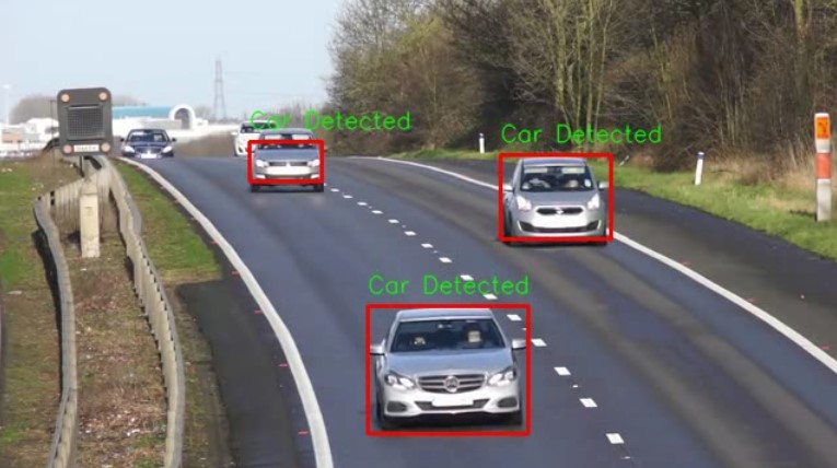
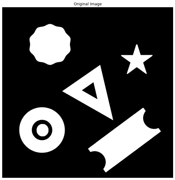
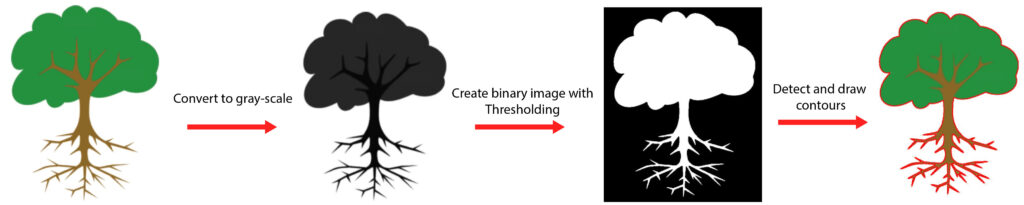
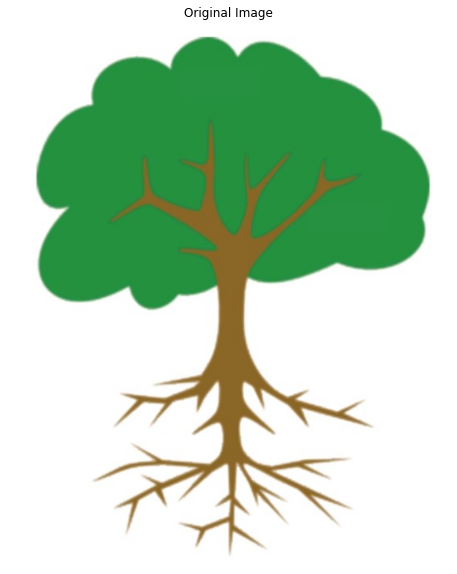
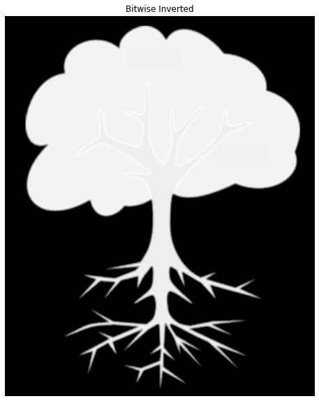
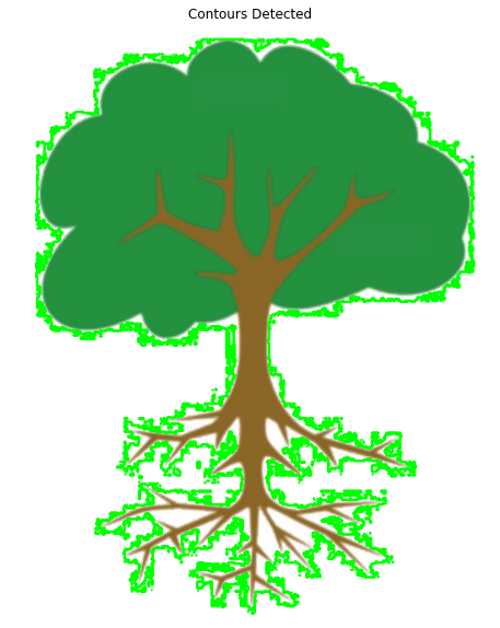
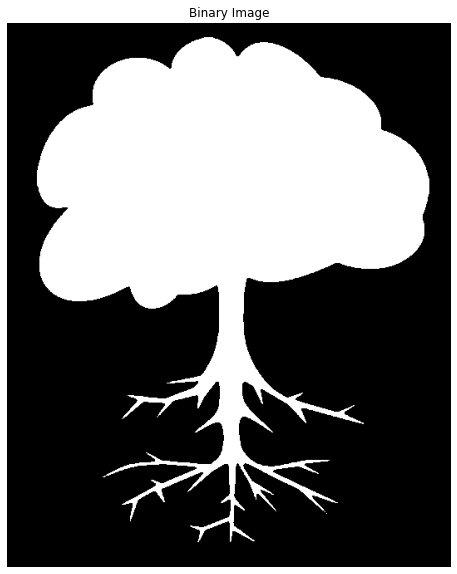
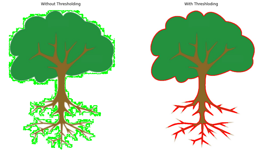
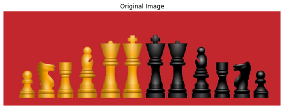
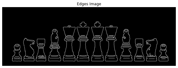
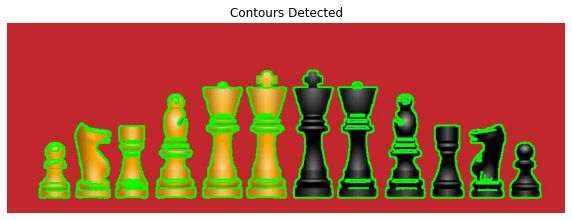
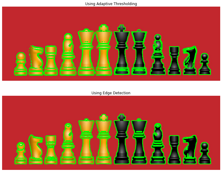
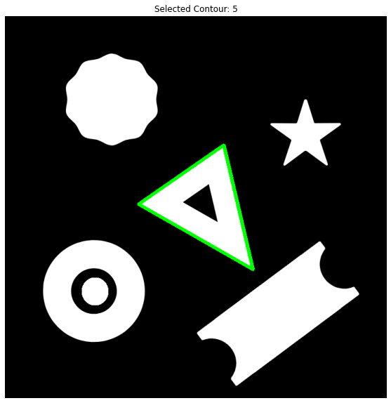
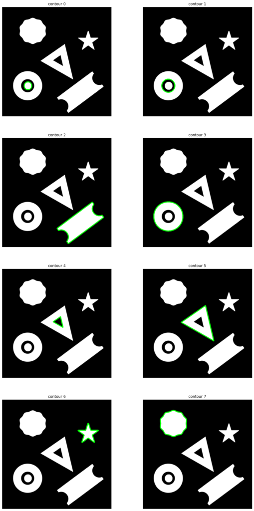
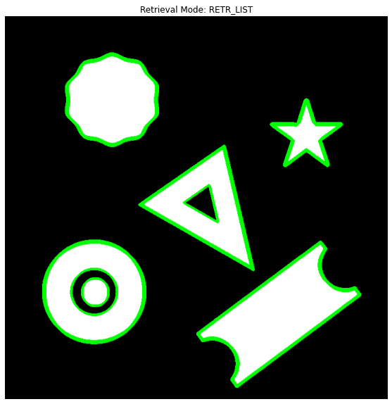
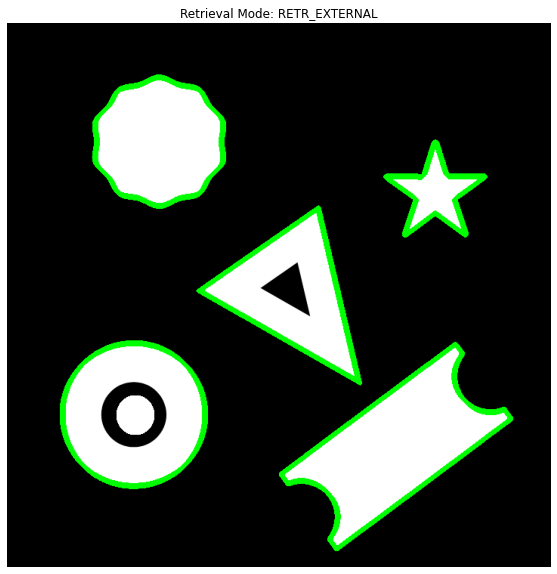
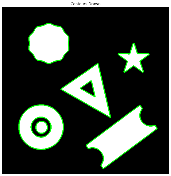
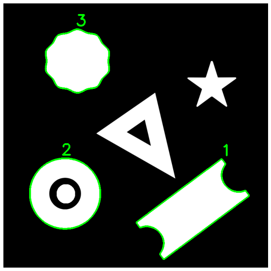
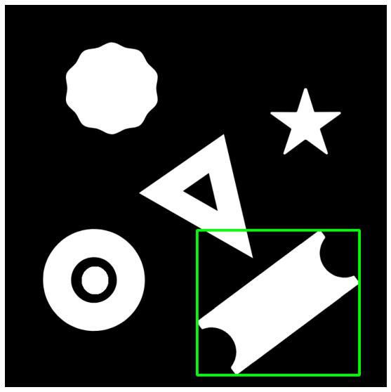
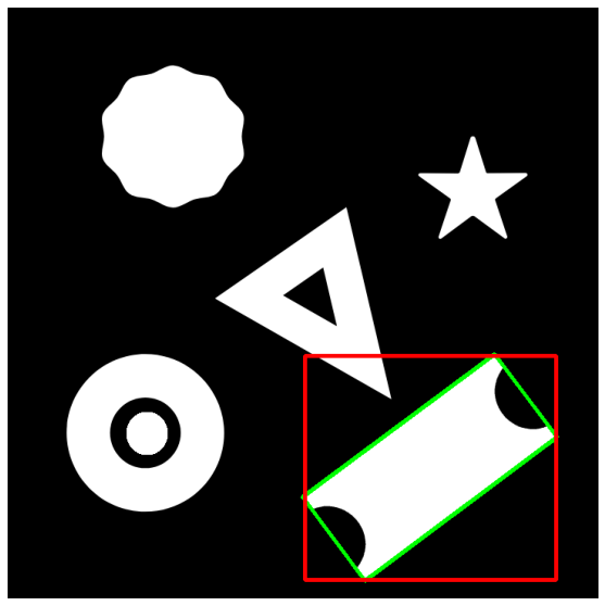
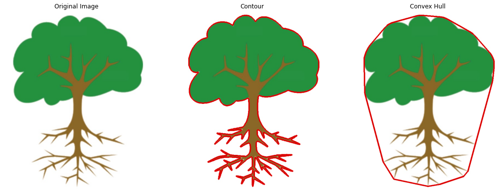
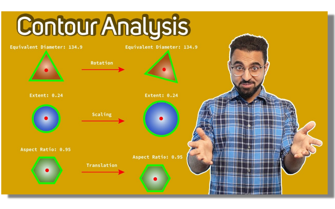
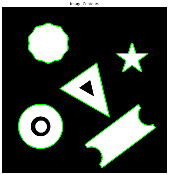
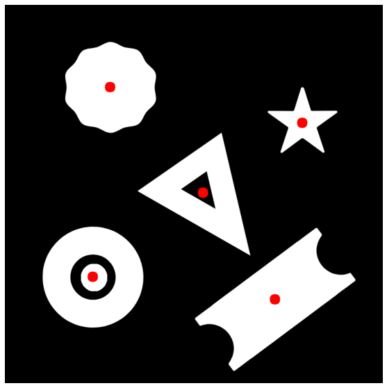
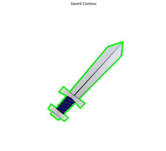
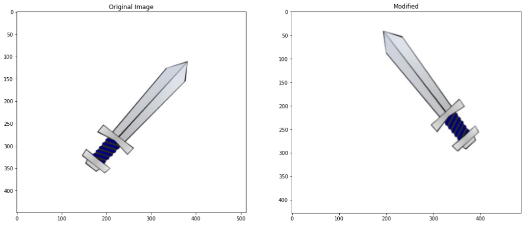
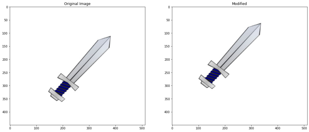
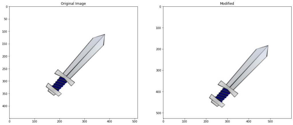
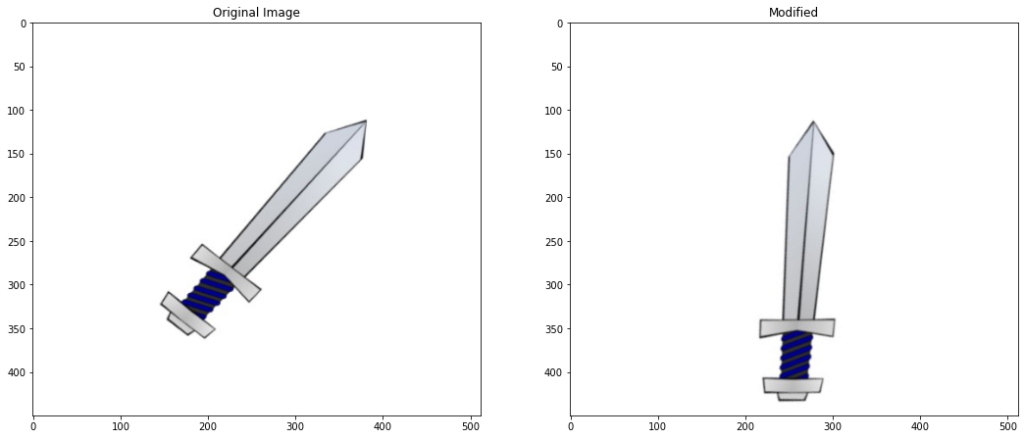
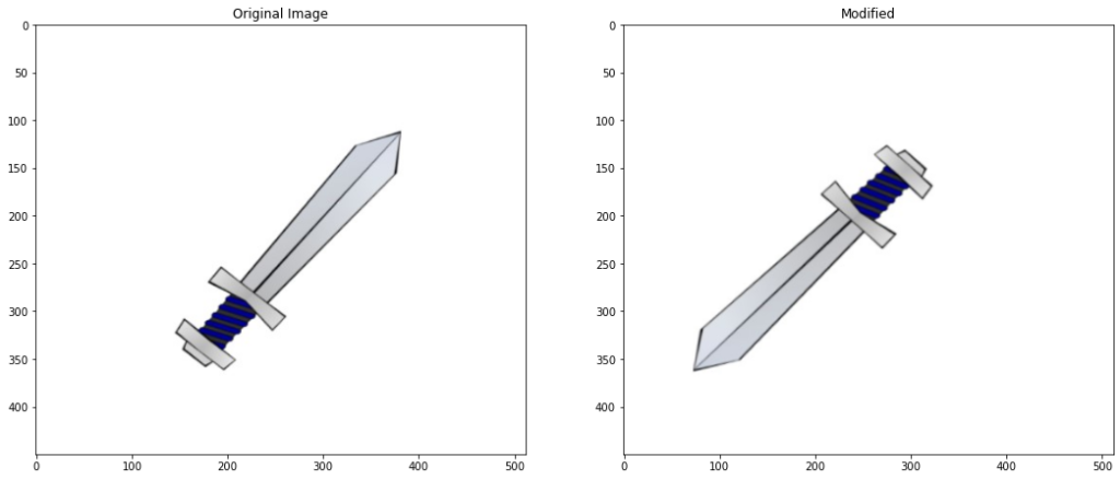
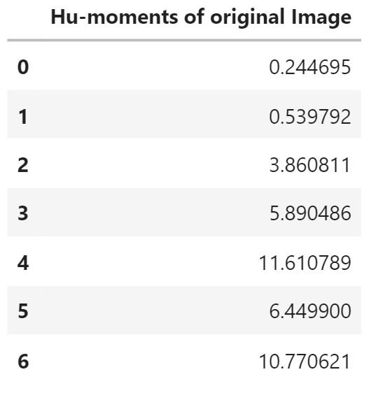
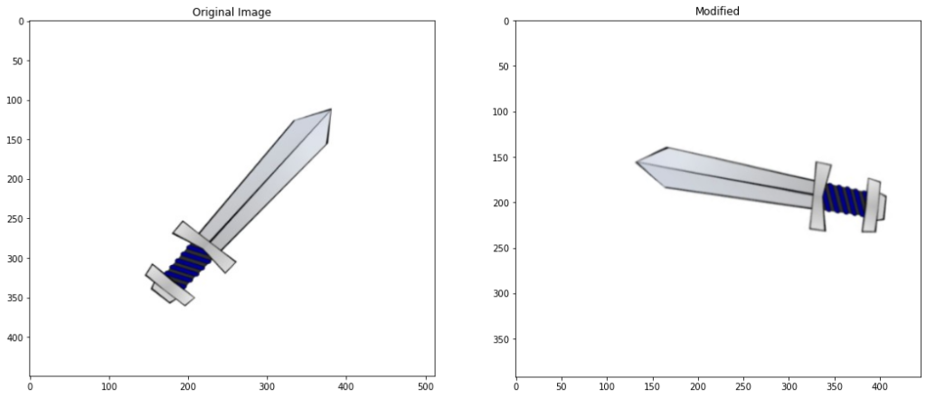
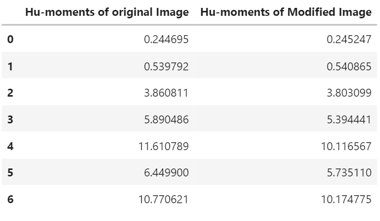
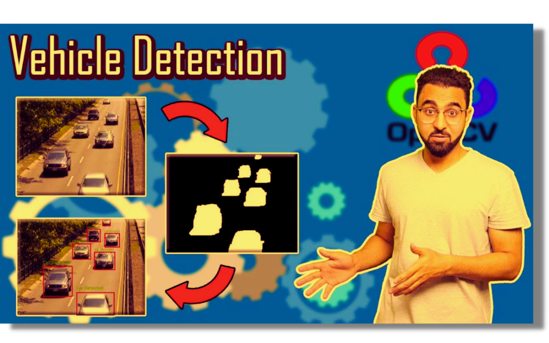
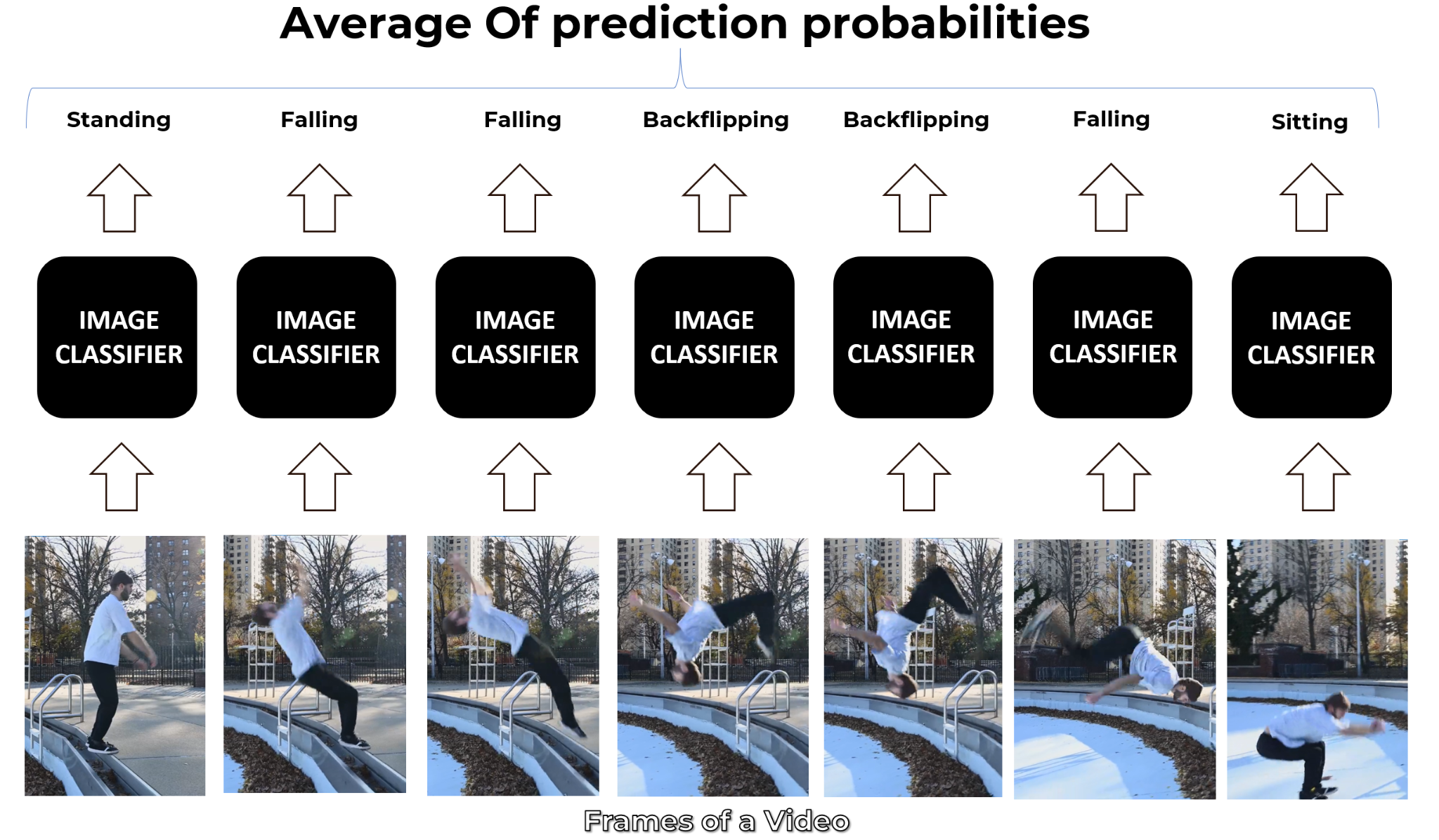
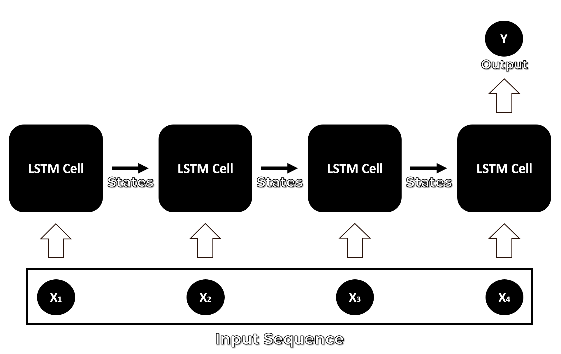
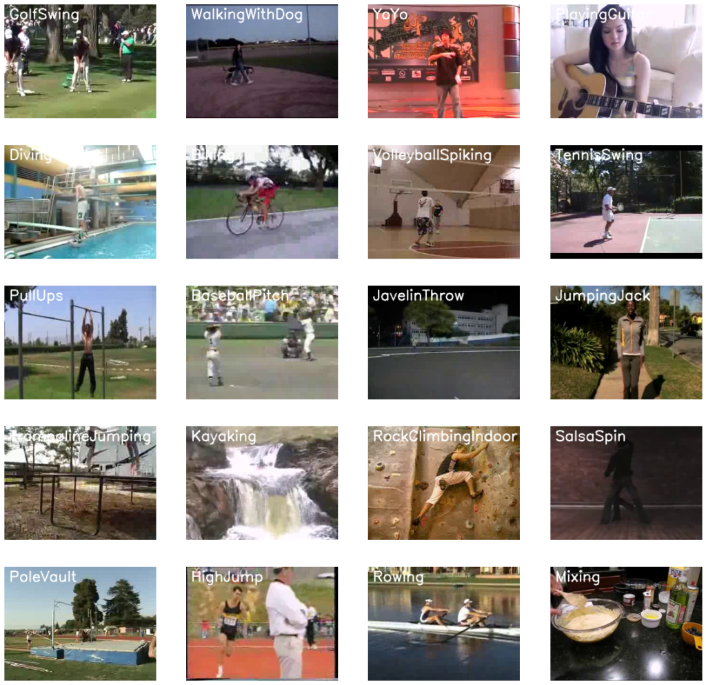
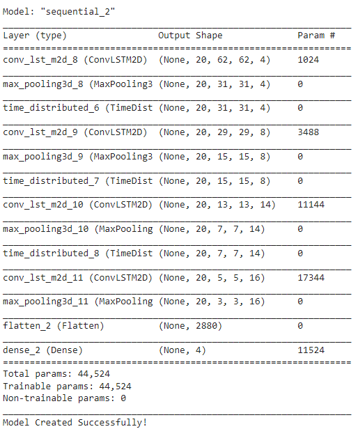
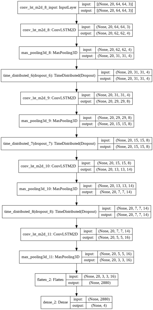
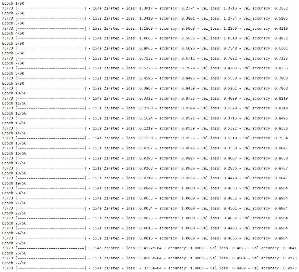
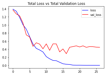
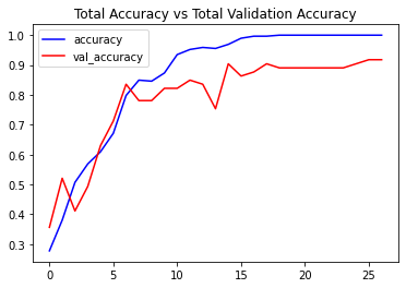
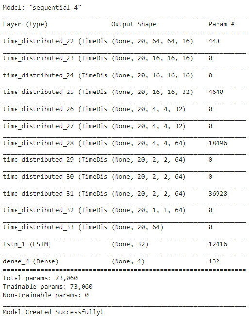
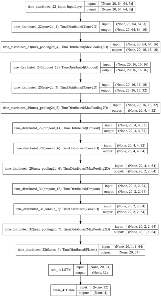
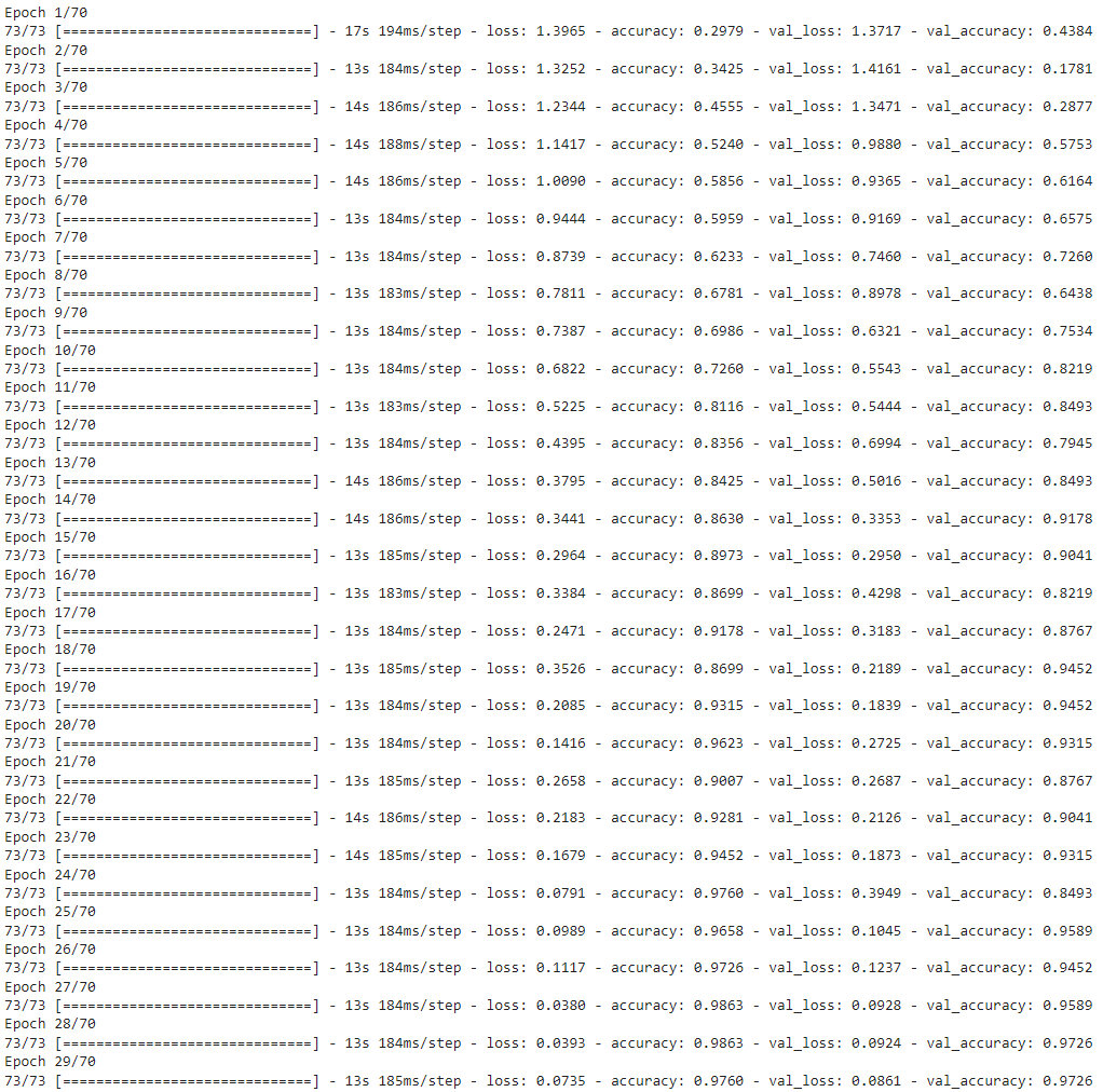
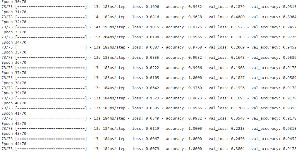
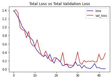
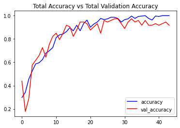
Let’s work together