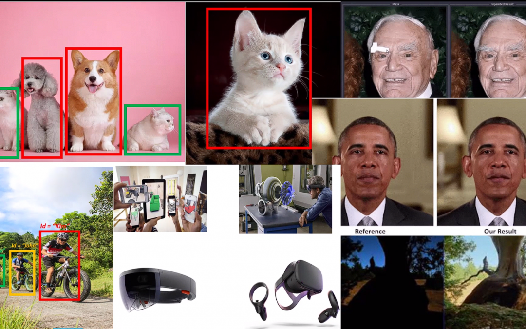
In this video I discuss different domains in vision, like Classification, detection, localization, tracking. Computational photography techniques like black hole imagery etc, amazing applications with GANS like deepfakes, image inpainting, Cycle Gans etc. I also talk about Geometrical Vision specifically 8 Different ways and techniques to Compute Depth. How Kinect v1 & v2 work and a lot lot more
I’m offering a premium 3-month Comprehensive State of the Art course in Computer Vision & Image Processing with Python (Urdu/Hindi). This course is a must take if you’re planning to start a career in Computer vision & Artificial Intelligence, the only prerequisite to this course is some programming experience in any language.
This course goes into the foundations of Image processing and Computer Vision, you learn from the ground up what the image is and how to manipulate it at the lowest level and then you gradually built up from there in the course, you learn other foundational techniques with their theories and how to use them effectively.
Hire Us
Let our team of expert engineers and managers build your next big project using Bleeding Edge AI Tools & Technologies
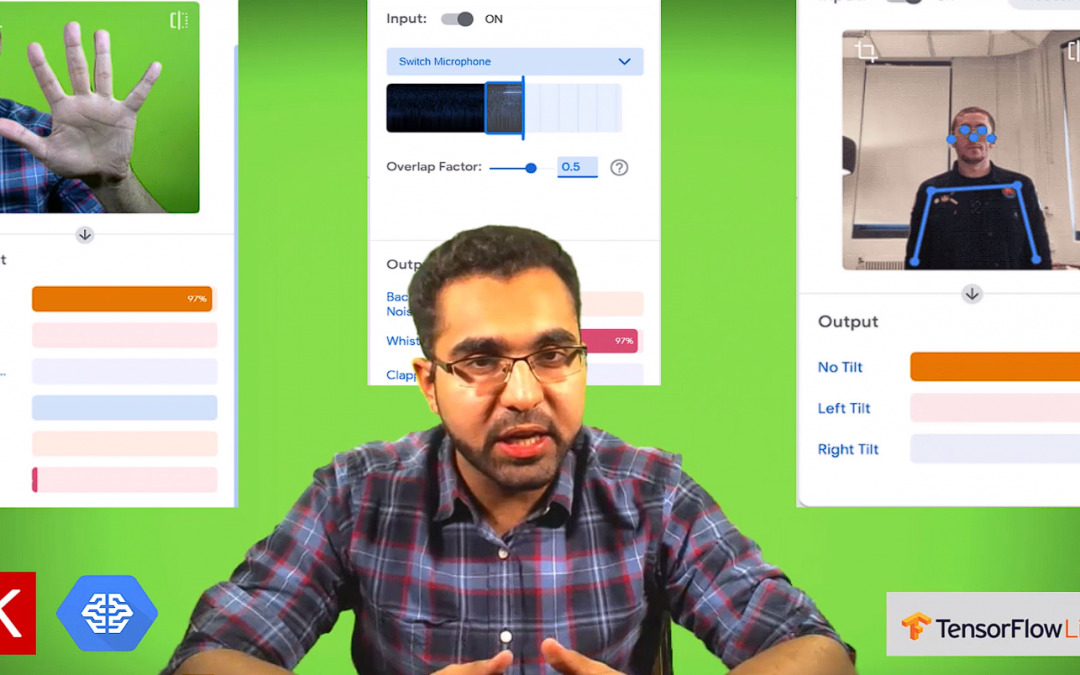
In less than 10 minutes I teach you how to train an effective hand finger recognition classifier, a pose detection model & a sound recognition model and also show you multiple deployment options.
If you’re not impressed yet than let me tell you this: “You won’t need any programming knowledge or need to install anything to work with this, an internet connection with a browser is sufficient.”
Unless you’re using Internet Explorer 😐
So the tool we are using is Teachable Machine version 2. A few months ago I made a video on Teachable machine version 1 but version 1 was more of a teaching tool. This version actually is a lot more powerful and allows you to export models in various ways.
I’m offering a premium 3-month Comprehensive State of the Art course in Computer Vision & Image Processing with Python (Urdu/Hindi). This course is a must take if you’re planning to start a career in Computer vision & Artificial Intelligence, the only prerequisite to this course is some programming experience in any language.
This course goes into the foundations of Image processing and Computer Vision, you learn from the ground up what the image is and how to manipulate it at the lowest level and then you gradually built up from there in the course, you learn other foundational techniques with their theories and how to use them effectively.
Hire Us
Let our team of expert engineers and managers build your next big project using Bleeding Edge AI Tools & Technologies
In this single tutorial alone I go over 5 different Google AI Experiments, I show you how you can use them inside the browser and how most of them essentially work. As these applications are openSource you will also get the GitHub repo for these experiments.
Some seasoned practitioners among you can even build on top of these applications and make something more interesting out of it.
I hope you found this tutorial useful. For future Tutorials by us, make sure to Subscribe to Bleed AI below
I’m offering a premium 3-month Comprehensive State of the Art course in Computer Vision & Image Processing with Python (Urdu/Hindi). This course is a must take if you’re planning to start a career in Computer vision & Artificial Intelligence, the only prerequisite to this course is some programming experience in any language.
This course goes into the foundations of Image processing and Computer Vision, you learn from the ground up what the image is and how to manipulate it at the lowest level and then you gradually built up from there in the course, you learn other foundational techniques with their theories and how to use them effectively.
Hire Us
Let our team of expert engineers and managers build your next big project using Bleeding Edge AI Tools & Technologies
This is a multipurpose tutorial because not only we will install TensorFlow 2.0 with GPU but we will also set up our Nvidia GPU for OpenCV source installation so that we can use our GPU with the OpenCV DNN module. The Blog post for source installation of OpenCV in windows can be accessed here.
Note: For this tutorial you must have an Nvidia Cuda compatible GPU & I’m also assuming that you already have python installed in your system, if not then you can go ahead and install anaconda distribution for python 3.7 here.
Alright Let’s Get Started
Step 0: Uninstall any program that says NVIDIA:
First of all to avoid any headaches down the road, you should uninstall any NVIDIA related programs or drivers, don’t worry I’ll show you how to install the latest drivers. In case you are pretty sure that you have the correct drivers installed then you don’t need to perform this step.
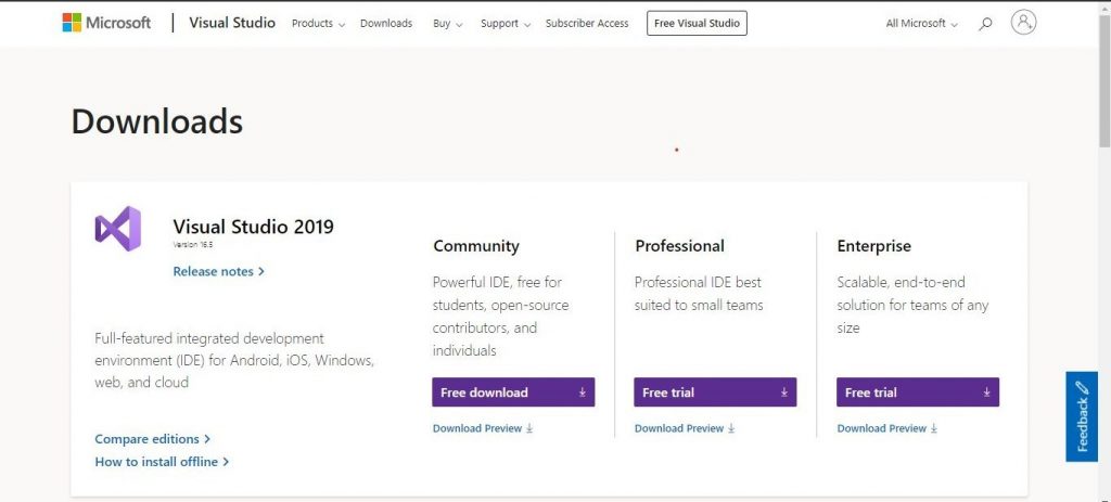
Step 1 (a): Download Visual Studio 2019:
Click here to download the Microsoft Visual Studio 2019 Community version
After Downloading you will get a .exe file.
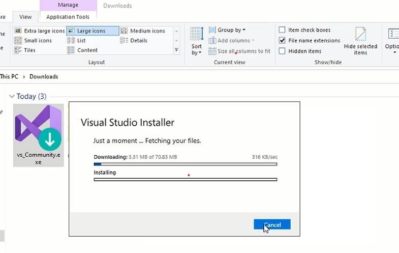
Step 1 (b): Install Visual Studio 2019
In order to begin the installation process click on the vs installer file and continue with default settings. After that downloading will begin and after downloading the installation process will start.
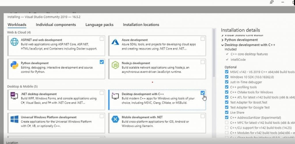
Step 1 (c): Select The Workloads in Visual Studio 2019
Finally, after completing the installation, you will be required to select workloads
As you can see above that we have SelectedPython Development and Desktop Development C++
Make sure to select Desktop development with c++ otherwise at the time of CMake compilation during OpenCV source installation you will get errors.
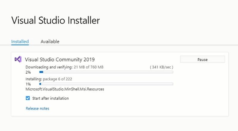
After Selecting the workloads Click the Install Button and your Packages will start downloading and then installing.
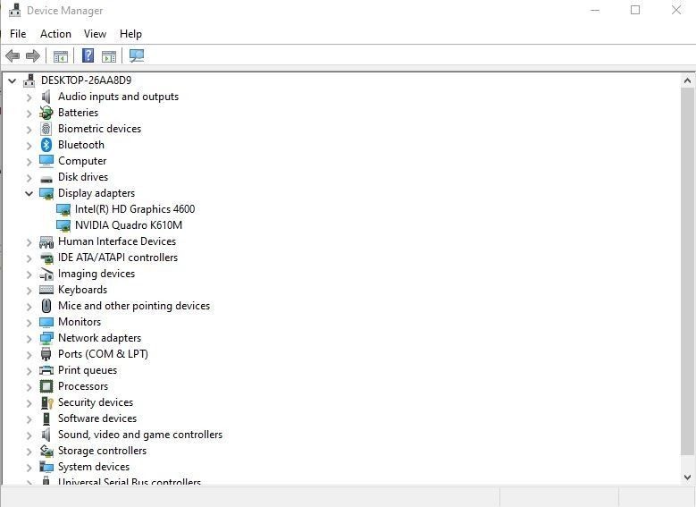
Step 2 (a): Check your Graphics Card.
Go to the device manager and under display adapters note down the name of your Nvidia Graphics card.
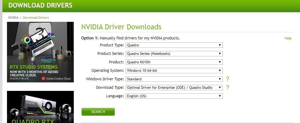
Step 2 (b): Download & Install the driver:
Now go to the Nvidia homepage here, and put your graphics card Operating system info as shown, I’m putting this information according to my card, for your card it will be different.
After this hit search & you will be able to download the driver.
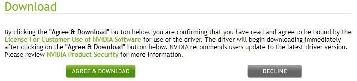
After downloading you have to launch the .exe file and install the driver, it’s a pretty smooth process. If you selected a wrong driver then it will tell you that during the installation.
Optionally if you’re confused you can also watch a video walkthrough of step 2a & step 2b here.
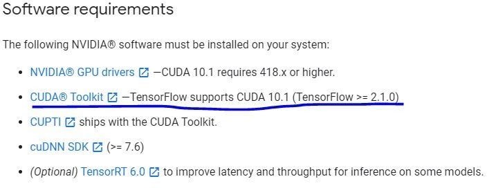
Step 3: Download & Install Cuda Toolkit:
Now you can head over to the TensorFlow GPU Support page here and see the latest required Cuda toolkit version for the TensorFlow GPU.
In my case, it’s Cuda version 10.1
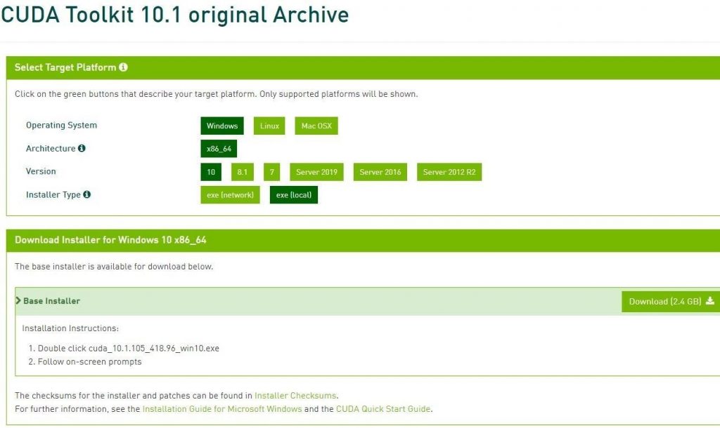
You can download the Cuda toolkit 10.1 version from here. I have selected my windows 10 and a .exe local file, Now you will download the 2.4 GB file.
After downloading the Cuda toolkit, run it through the installation process.
Step 4 (a): Download CudNN:
Now you need to download cudNN but before you can do that you need to make an account on NVIDIA, so first make an account here.
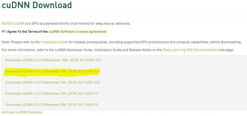
After you have made the account you can download cuDNN from here. Note Download the correct compatible version of cudNN for your associated Cuda toolkit version, for e.g. I will be downloading cuDNN v7.6.5, for CUDA 10.1 which is compatible with Cuda toolkit version 10.1
Step 4 (b): Configure CuDNN:
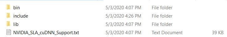
After downloading the cuDNN zip folder, extract it and then you will have 3 folders bin, include & lib like this:
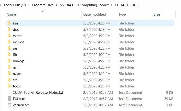
Now navigate to where you installed Cuda 10.1 toolkit. For me, the path was this: C:\Program Files\NVIDIA GPU Computing Toolkit\CUDA\v10.1
Inside v10.1 directory you will see these folders there:
Now what you will do is take the contents of the bin, include & lib folders inside of cuDNN unzipped folder and put it inside the bin, include & lib folders of v10.1 directory.
So you will take the file cudnn64_7.dll (from the bin folder of cuDNN) and put it inside the bin folder of v10.1.
Then you will take cudnn.ln (from include folder of cuDNN) and put it inside the include folder of v10.1.
Then you will take cudnn.lib (from lib/64 folder of cuDNN) and put it inside lib/x64/ folder of v10.1.
Don’t worry if you are confused, I will give you a video walkthrough the link of this step.
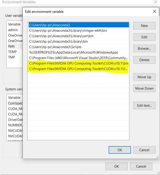
Step 4 (c): Add Paths to Environment variables.
The next step is to add the path to your bin folder inside v10.1 and libnvvp to the path variable inside user variables in the Environment variables.
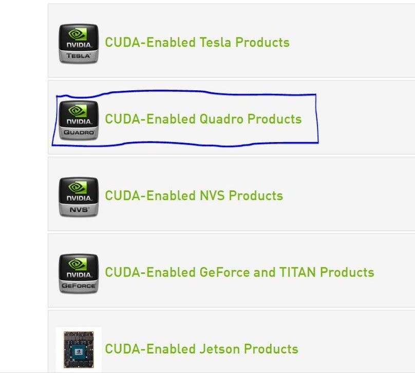
Find your exact GPU name and note the compute capability, the compute capability is the architecture version which we will be using during the installation of OpenCV from Source.
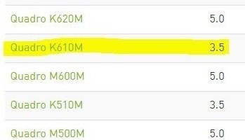
Since I’m using a Quadro k610M GPU on my laptop, I’ll search for my GPU under Cuda-Enabled Quadro Products.
Now by searching I can see that my architecture version is: 3.5, this is a pretty low number but hey I’m not using a big machine here.
And That’s it
I’m offering a premium 3-month Comprehensive State of the Art course in Computer Vision & Image Processing with Python (Urdu/Hindi). This course is a must take if you’re planning to start a career in Computer vision & Artificial Intelligence, the only prerequisite to this course is some programming experience in any language.
This course goes into the foundations of Image processing and Computer Vision, you learn from the ground up what the image is and how to manipulate it at the lowest level and then you gradually built up from there in the course, you learn other foundational techniques with their theories and how to use them effectively.
Hire Us
Let our team of expert engineers and managers build your next big project using Bleeding Edge AI Tools & Technologies
In this post we are going to install OpenCV from Source in Windows 10. OpenCV stands for Open Source Computer Vision library. It’s the most widely used and powerful computer vision & Image processing library in the world. It has been around for more than 20 years and contains 1000s of Optimized algorithms written in C++ and has bindings in other languages like python, java, etc.
Now if this is your first time dealing with OpenCV then I would highly recommend that instead of following this tutorial and installing from source, you just install OpenCV with pip by doing:
pip install opencv-contrib-python
Now if you have already used OpenCV in the past and want to have more control over how this library gets installed in your system then source installation is the way to go. By now you have realized that there are two ways to go about installing this library, one is the installation with a package manager like pip or conda, the other is an installation from source.
Now before we start with installing from source, you first need to understand what are the advantages vs disadvantages when you are installing from source vs with a package manager.
Installation with Package Manager (pip/conda):
Advantages:
The installation is really easy, you just have to run a single line of command. No extra knowledge required.
You can easily update the library with a single line too.
Disadvantages:
This method will install features that are preset by the library maintainers, these will be the most commonly used features. The programmer doesn’t have the ability to select features of his/her own choice.
The programmer can’t do any extra optimization by selecting different available Optimization flags.
Installation from Source:
Advantages:
The method allows you to add your own features or get rid of already present features, this is especially useful when you want to use a feature which does not come with the default installation or when you are deploying on a device with limited memory so then you can get rid of unnecessary features.
You can select some Optimization flags and get fast performance in some areas of the library.
Disadvantages:
The installation is a tedious process, many things along the way can go wrong.
To work with the flags you must be familiar with the library so you know which features to enable or disable for your specific purpose.
In order to update you have to do more than just run a single line of command.
In this tutorial the two main advantages from source installation that you will get, first you will be able to enable the Non-Free Algorithms in OpenCV. In later versions of OpenCV you can’t use algorithms like SIFT, SURF, etc as they are not installed with pip, but with source installation you will be able to install these. You will also be able to enable Cuda flags so that you can use Nvidia GPUs with the OpenCV DNN module, which will give you a huge speed boost when running neural nets in OpenCV. You can still follow along if you don’t have an Nvidia GPU, you will just have to skip that part.
Step 0: Uninstall OpenCV (Do this only if you already have OpenCV installed)
If you are installing OpenCV in your system for the first time then you can ignore this step but if you already have installed OpenCV in your system then this step is for you.
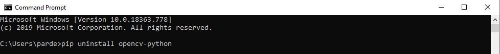
Open up the command prompt and do:
pip uninstall opencv-python
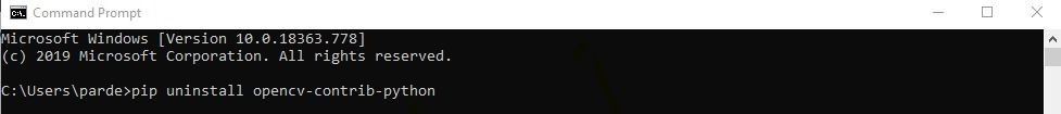
And also do
pip uninstall opencv-contrib-python
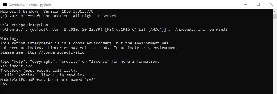
After Uninstalling these then you should see an error when you import OpenCV by doing: import cv2
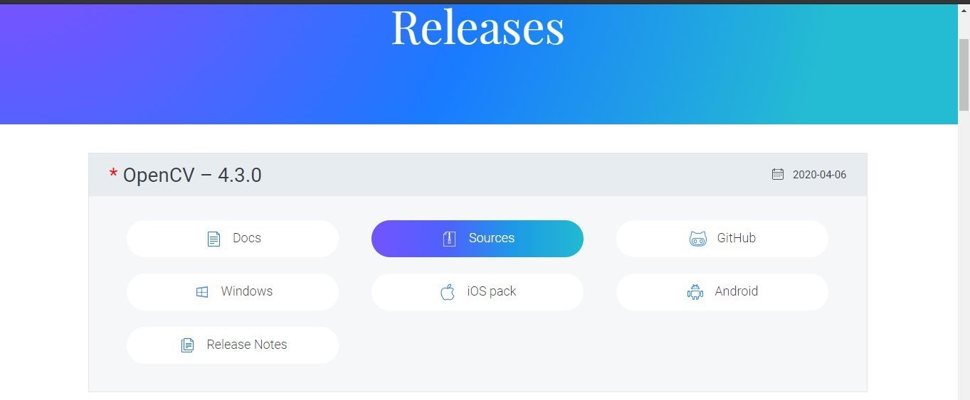
Click on the Sources button, and you’ll download a zip folder named opencv-4.3.0.zip
Make a new folder named “OpenCV-Installation” and extract this zip folder inside that folder. You can then get rid of the zip folder now.
Step 2: Download OpenCV contrib Package
The contrib package in OpenCV gives you a lot of other interesting modules that you can use with but unfortunately it does not come with the default installation so we have to download it from Github. Download the Source code (zip)
from here and Unzip it in the OpenCV-Installation directory. Note: It’s not required to unzip here but this way it will be cleaner.
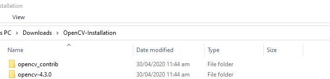
After Unzipping both folders my Opencv-installation directory looks like this
So what we just did is that we created a folder named OpenCV- Installation and inside this folder we put opencv_contrib (Extracted) and opencv-4.3.0 (Extracted).
Step 3 (a): Download Visual Studio 2019
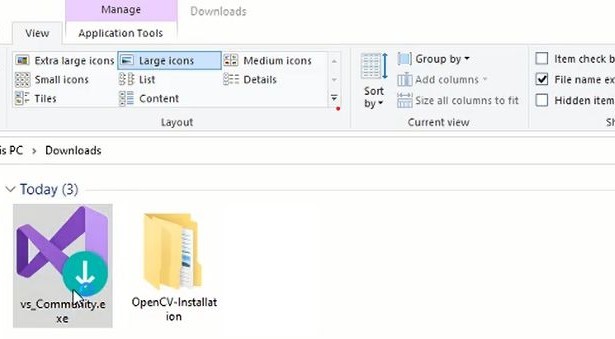
Click here to download the Microsoft Visual Studio 2019 Community version
After Downloading you will get
Step 3 (b): Install Visual Studio 2019
In order to begin the installation process click on the vs installer file and continue with default settings. After that downloading will begin and after downloading the installation process will start
Step 3 (c): Select The Workloads in Visual Studio 2019
Finally, after completing the installation, you will be required to select workloads
As you can see above that we have SelectedPython Development and Desktop Development C++
Note: if you are using the only python you would still need to select Desktop development with c++ otherwise at the time of CMake compilation of OpenCV you will get errors.
After Selecting the workloads Click the Install Button and your Packages will start downloading and then installing.
Step 4: Download and Install CMake
Now we have to download & install CMake. CMake is open-source software designed to build packages in a compiler-independent manner. During the installation of OpenCV from source, CMake will help us to control the compilation process and it will generate native makefiles and workspaces. For more information about CMake you can look here.
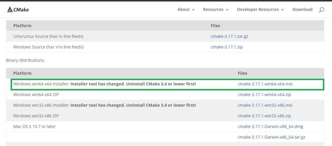
Click here and download the latest version of CMake, In our case, we are downloading CMake-3.17.1.
Open the Installer file and Begin the installation but on the time of installation you’ll be asked 3 things
Agree with the terms & conditions (checkmark).
Do you want to add CMake to the system path, if you were going to use CMake with the command line then you should check this but since we’re going to be using the CMake GUI for configuration so we don’t need to check this for now.
Lastly, it will ask if you want to change the installation location (Keep it as default).
Step 5: Setting up CMake for Compilation
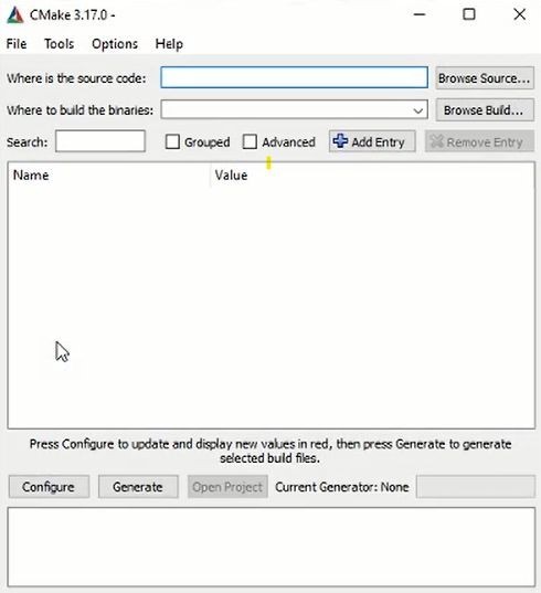
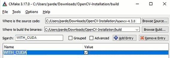
After completion of installation. Go to the Start Menu and type CMake in the search tab, click on it, you will get this window
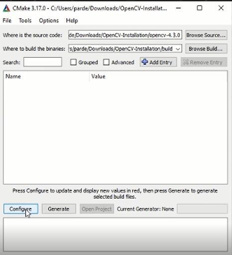
Where is the Source code: Select the Opencv installation file OpenCV-4.3.0 which you just put inside the OpenCV-Installation directory.
Where to build the binaries: This is where the build binaries will be saved, if a path does not exist (which will be true when you’re running this the first time) then CMake will ask you and then create it. For our case, we are just setting the path to be our OpenCV-installation directory followed by `/build`
It would look something like this:
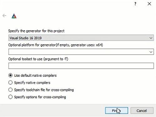
And after selecting both paths Click on the Configure button also Keep the setting as default and click on the Finish button.
Step 6 (a): Setting up Required Flags for our Installation
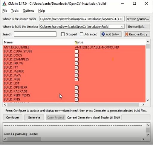
After compilation a window like this will appear, which allows you to select flags that you want. Now by checking these flags or unchecking them you will have a customized installation of OpenCV. If you were doing a pip installation then you wouldn’t have this ability.
Checking each flag adds more functionality/modules etc to your OpenCV installation.
For this OpenCV installation a lot of flags are already checked but we’ll checkmark some more flags to include them and we will also provide the path of opencv-contrib package in order to use the modules that are present in opencv-contrib Package.
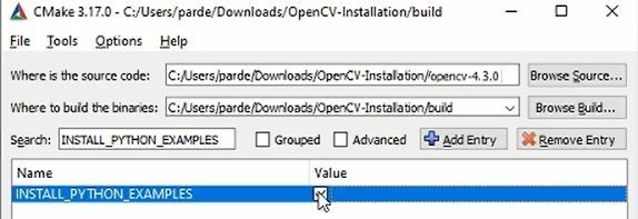
1. INSTALL_PYTHON_EXAMPLES
This flag enables the installation of the Python examples present in the sample folder created during the extraction of the OpenCV zip.
In Search bar write INSTALL_PYTHON_EXAMPLES and check-mark it, like this:
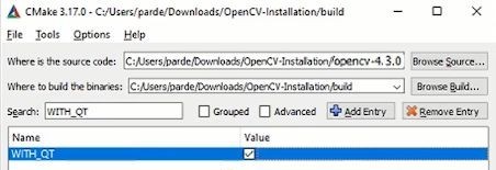
2. WITH_QT
Qt is a cross-platform app development framework for desktop, embedded systems, and mobile. With Qt, you can write GUIs directly in C++ using its Widgets modules. Qt is also packaged with an interactive graphical tool called Qt Designer which functions as a code generator for Widgets based GUIs.
In Search bar write WITH_QT and checkmark it, like this:
3. WITH_OPENGL
This will allow OpenGL support in OpenCV for building applications related to OpenGL. OpenGL is used to render 3D scenes. These 3D scenes can be later processed using OpenCV.
In Search bar write WITH_OPENGL and check mark it, like this:
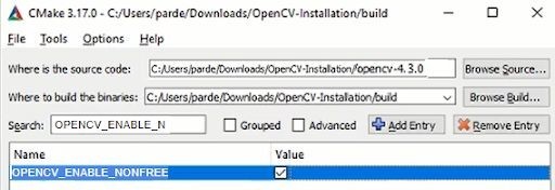
4. OPENCV_ENABLE_NONFREE
This will allow us to use those Non-Free algorithms like SIFT & SURF.
In Search bar write OPENCV_ENABLE_NONFREE and checkmark it, like this:
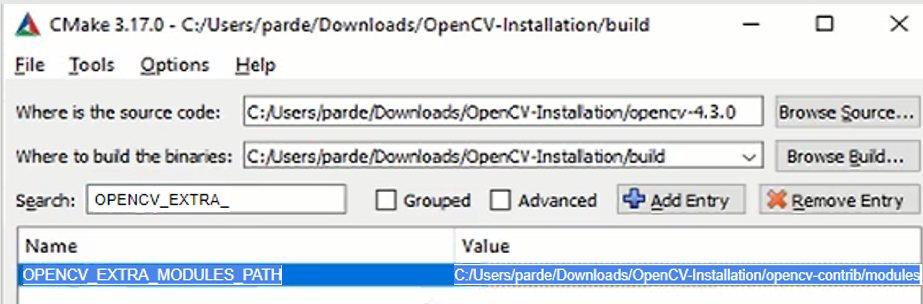
5. OPENCV_EXTREA_MODULES_PATH
To finally include the opencv contrib package that you downloaded in step 2 in OpenCV you would need to add its path to the OPENCV_EXTRA_MODULES_PATH flag.
In Search bar write OPENCV_EXTRA_MODULES_PATH and provide a path of opencv- contrib package, like this:
In our case the path is: C:/Users/parde/Downloads/OpenCV-Installation/opencv-contrib/modules
Note: In my system I had to replace backward slashes with forward slashes in the above path to avoid an error, this might not be the case with you.
Step 6 (b): Setting up Nvidia GPUs & Enable cuda flags.
Now if you don’t have an Nvidia GPU then please skip this step and go to step 6c. If you do have an Nvidia GPU then there are two parts to make this work. The first part is to install Cuda drivers, toolkit & cudnn and the second is to enable Cuda flags.
Part 1: Install Cuda Drivers, Cuda Toolkit & Cudnn:
Since the first part itself is long and many of you who have Nvidia GPUs may already have done most of that installationso I’m covering it in another blog post here, this post also lets you install TensorFlow 2.0 GPU in your system.
Part 2: Enable Cuda Flags:
After you have completed part 1, you can enable the below flags.
1. WITH_CUDA
This option allows CUDA support in the OpenCV. You need to make sure that you have CUDA enabled GPU in your machine in order to use the CUDA library.
In Search bar write WITH_CUDA and checkmark it, like this:
2. OPENCV_DNN_CUDA
Also enable opencv_dnn_cuda flag.
In Search bar write OPENCV_DNN_CUDA and checkmark it, like this:
3. CUDA_ARCH_BIN
Now enter your Cuda architecture version that you found out at the end of the post linked in part 1 step 6(b), it’s important that you enter the correct version.
In Search bar write CUDA_ARCH_BIN and checkmark it, like this:
Note: In some cases I’ve noticed due to some reason the CUDA_ARCH_BIN flag is not visible until you press the configure button, so press the configure button and then put the value of this flag and then you have to again press the configure button in step 6c.
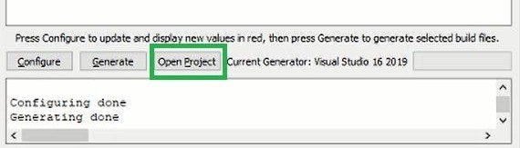
Step 6 (c): Configure & Generate
Click on the Configure button. After completion you will get this message:
After Configuration is done press the generate button.
Step 7: Build the Libraries in Visual Studio
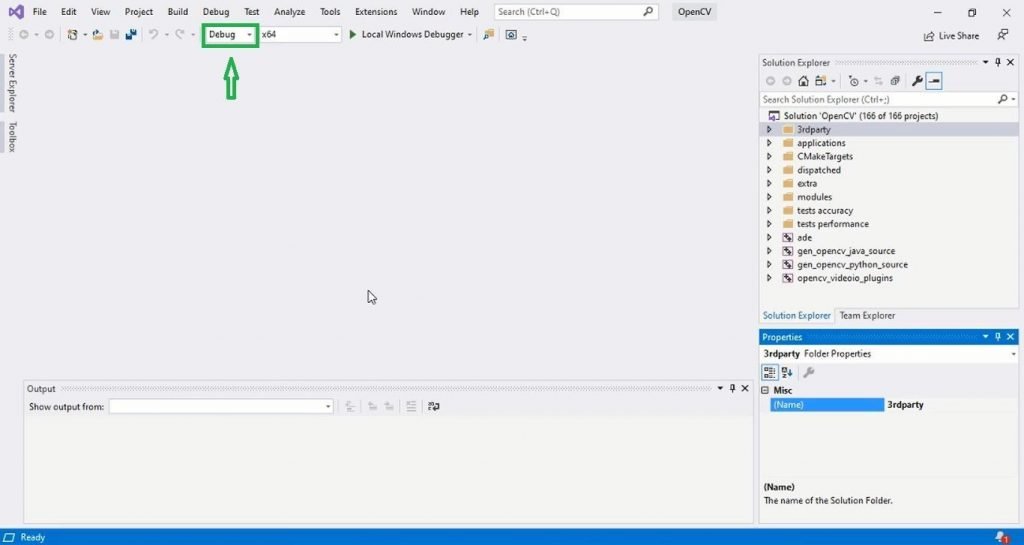
In Order to build the libraries you need to open up OpenCV.sln which will be in your build folder or you can open it up by clicking the Open Project button on the CMake window.
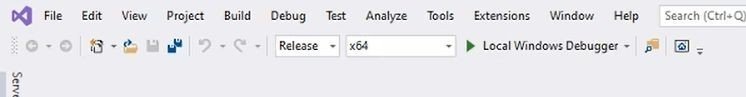
After clicking the Open Project button you will get this window change the Debug mode to Release mode. Don’t forget this step.
After changing to Release mode:
And now it’s time to install the libraries
Expand the CMake Target directory which is on the right side of your screen.
Right Click on ALL_BUILD
Click the build option
It will take time to build the libraries, the time of building depends upon what and how many flags you enabled. If you have enabled Cuda flags it may take several hours to build.
After the build is finished you will get this message.
If you see this message it means that your build was successful.
Step 8: Install the Library in Visual Studio
Below the ALL_BUILD file, you will see an INSTALL file
Right Click on the INSTALL file
Click on the build option
Your installation will begin, and at the `end of the build you will get this message
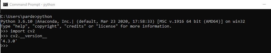
Step 9: Verify the Installation of OpenCV
Open the cmd terminal and run the Python Interpreter and then type
import cv2 (Hit Enter)
cv2.__version__ (Hit Enter)
if your output is the same as the screenshot below then your installation went good.
Congratulations! Your Installation Is Complete 🙂
Using GPUs with OpenCV DNN Module:
For those of you that have installed OpenCV with GPU support might be wondering how to use it.
Now if you have never worked with the DNN Module then I would recommend that you take a look at the coding part of our Super Resolution blog post.
So for e.g. if you wanted to run the above code on an Nvidia GPU then you just need to include 2 lines after you read the model and its configuration file with readNet function.
These lines must come before the forward pass is performed and that’s it. If you have configured everything properly then OpenCV will utilize your Nvidia GPU to run the network in the forward pass.
Also as a bonus tip, if you wanted to use OpenCL based GPU in your system then instead of those two lines you can use this line:
By running your models in Nvidia GPU or Intel-based GPU, you will find a tremendous speed increase, provided of course you have a strong GPU. If you didn’t install with GPU support then by putting these lines it wouldn’t use the GPU but it won’t give an error either.
In Our Computer Vision & Image processing Course (Urdu/Hindi) I actually go over 13-14 different neural nets with OpenCV DNN and provide you coding examples & Video Walkthroughs to use all of them with the Nvidia and OpenCL based GPUs. Besides that the course itself is pretty comprehensive and arguably one of the best if you want to start a career in Computer Vision & Artificial Intelligence, the only prerequisite to this course is some programming experience in any language.
This course goes into the foundations of Image processing and Computer Vision, you learn from the ground up what the image is and how to manipulate it at the lowest level and then you gradually built up from there in the course, you learn other foundational techniques with their theories and how to use them effectively.
You can reach out to me personally for a 1 on 1 consultation session in AI/computer vision regarding your project. Our talented team of vision engineers will help you every step of the way. Get on a call with me directlyhere.