Convolutional Neural Networks (CNN) are great for image data and Long-Short Term Memory (LSTM) networks are great when working with sequence data but when you combine both of them, you get the best of both worlds and you solve difficult computer vision problems like video classification.
In this tutorial, we’ll learn to implement human action recognition on videos using a Convolutional Neural Network combined with a Long-Short Term Memory Network. We’ll actually be using two different architectures and approaches in TensorFlow to do this. In the end, we’ll take the best-performing model and perform predictions with it on youtube videos.
Before I start with the code, let me cover some theories on video classification and different approaches that are available for it.
Image Classification
You may already be familiar with an image classification problem, where, you simply pass an image to the classifier (either a trained Deep Neural Network (CNN or an MLP) or a classical classifier) and get the class predictions out of it.
But what if you have a video? What will happen then?
Before we talk about how to go about dealing with videos, let’s just discuss what videos are exactly.
But First What Exactly Videos are?
Well, so it’s no secret that a video is just a sequence of multiple still images (aka. frames) that are updated really fast creating the appearance of a motion. Consider the video (converted into .gif format) below of a cat jumping on a bookshelf, it is just a combination of 15 different still images that are being updated one after the other.
Now that we understand what videos are, let’s take a look at a number of approaches that we can use to do video classification.
Approach 1: Single-Frame Classification
The simplest and most basic way of classifying actions in a video can be using an image classifier on each frame of the video and classify action in each frame independently. So if we implement this approach for a video of a person doing a backflip, we will get the following results.
The classifier predicts Falling in some frames instead of Backflipping because this approach ignores the temporal relation of the frames sequence. And even if a person looks at those frames independently he may think that the person is Falling.
Now a simple way to get a final prediction for the video is to consider the most frequent one which can work in simple scenarios but is Falling in our case and is not correct. So another way to go about this is to take an average of the probabilities of predictions and get a more robust final prediction.
You should also check another Video Classification and Human Activity Recognition tutorial I had published a while back, in which I had discussed a number of other approaches too and implemented this one using a single-frame CNN with moving averages and it had worked fine for a relatively simpler problem.
But as mentioned before, this approach is not effective, because it does not take into account the temporal aspect of the data.
Approach 2: Late Fusion
Another slightly different approach is late fusion, in which after performing predictions on each frame independently, the classification results are passed to a fusion layer that merges all the information and makes the prediction. This approach also leverages the temporal information of the data.
This approach does give decent results but is still not powerful enough. Now before moving to the next approach let’s discuss what Convolutional Neural Networks are. So that you get an idea of what that black box named image classifier was, that I was using in the images.
Convolutional Neural Network (CNN)
A Convolutional Neural Network (CNN or ConvNet) is a type of deep neural network that is specifically designed to work with image data and excels when it comes to analyzing the images and making predictions on them.
It works with kernels (called filters) that go over the image and generates feature maps (that represent whether a certain feature is present at a location in the image or not) and initially it generates few feature maps and as we go deeper in the network the number of feature maps is increased and the size of maps is decreased using pooling operations without losing critical information.
Each layer of a ConvNet learns features of increasing complexity which means, for example, the first layer may learn to detect edges and corners, while the last layer may learn to recognize humans in different postures.
Now let’s get back to discussing other approaches for video classification.
Approach 3: Early Fusion
Another approach of video classification is early fusion, in which all the information is merged at the beginning of the network, unlike late fusion which merges the information in the end. This is a powerful approach but still has its own limitations.
Approach 4: Using 3D CNN’s (aka. Slow Fusion)
Another option is to use a 3D Convolutional Network, where the temporal and spatial information are merged slowly throughout the whole network that is why it’s called Slow Fusion. But a disadvantage of this approach is that it is computationally really expensive so it is pretty slow.
Approach 5: Using Pose Detection and LSTM
Another method is to use a pose detection network on the video to get the landmark coordinates of the person for each frame in the video. And then feed the landmarks to an LSTM Network to predict the activity of the person.
There are already a lot of efficient pose detectors out there that can be used for this approach. But a disadvantage of using this approach is that you discard all the information other than the landmarks, like the environment information can be very useful, for example for playing football action category the stadium and uniform info can help the model a lot in predicting the action accurately.
Before going to the approach that we will implement in this tutorial, let’s briefly discuss what are Long Short Term Memory (LSTM) networks, as we will be using them in the approach.
Long Short Term Memory (LSTM)
An LSTM network is specifically designed to work with a data sequence as it takes into consideration all of the previous inputs while generating an output. LSTMs are actually a type of neural network called Recurrent Neural Network, but RNNs are not known to be effective for dealing with the Long term dependencies in the input sequence because of a problem called the Vanishing gradient problem.
LSTMs were developed to overcome the vanishing gradient and so an LSTM cell can remember context for long input sequences.
Many-to-one LSTM network
This makes an LSTM more capable of solving problems involving sequential data such as time series prediction, speech recognition, language translation, or music composition. But for now, we will only explore the role of LSTMs in developing better action recognition models.
Now let’s move on towards the approach we will implement in this tutorial to build an Action Recognizer. We will use a Convolution Neural Network (CNN) + Long Short Term Memory (LSTM) Network to perform Action Recognition while utilizing the Spatial-temporal aspect of the videos.
Approach 6: CNN + LSTM
We will be using a CNN to extract spatial features at a given time step in the input sequence (video) and then an LSTM to identify temporal relations between frames.
The two architectures that we will be using to use CNN along with LSTM are:
ConvLSTM
LRCN
Both of these approaches can be used using TensorFlow. This tutorial also has a video version as well, that you can go and watch for a more detailed overview of the code.
Alright, so without further ado, let’s get started.
Import the Libraries
We will start by installing and importing the required libraries.
# Install the required libraries.
!pip install pafy youtube-dl moviepy
# Import the required libraries.
import os
import cv2
import pafy
import math
import random
import numpy as np
import datetime as dt
import tensorflow as tf
from collections import deque
import matplotlib.pyplot as plt

from moviepy.editor import *
%matplotlib inline

from sklearn.model_selection import train_test_split

from tensorflow.keras.layers import *
from tensorflow.keras.models import Sequential
from tensorflow.keras.utils import to_categorical
from tensorflow.keras.callbacks import EarlyStopping
from tensorflow.keras.utils import plot_model
And will set Numpy, Python, and Tensorflow seeds to get consistent results on every execution.
Step 1: Download and Visualize the Data with its Labels
In the first step, we will download and visualize the data along with labels to get an idea about what we will be dealing with. We will be using the UCF50 – Action Recognition Dataset, consisting of realistic videos taken from youtube which differentiates this data set from most of the other available action recognition data sets as they are not realistic and are staged by actors. The Dataset contains:
50 Action Categories
25 Groups of Videos per Action Category
133 Average Videos per Action Category
199 Average Number of Frames per Video
320 Average Frames Width per Video
240 Average Frames Height per Video
26 Average Frames Per Seconds per Video
Let’s download and extract the dataset.
# Discard the output of this cell.
%%capture

# Downlaod the UCF50 Dataset
!wget --no-check-certificate https://www.crcv.ucf.edu/data/UCF50.rar

#Extract the Dataset
!unrar x UCF50.rar
For visualization, we will pick 20 random categories from the dataset and a random video from each selected category and will visualize the first frame of the selected videos with their associated labels written. This way we’ll be able to visualize a subset ( 20 random videos ) of the dataset.CodeText
# Create a Matplotlib figure and specify the size of the figure.
plt.figure(figsize = (20, 20))

# Get the names of all classes/categories in UCF50.
all_classes_names = os.listdir('UCF50')

# Generate a list of 20 random values. The values will be between 0-50,
# where 50 is the total number of class in the dataset.
random_range = random.sample(range(len(all_classes_names)), 20)

# Iterating through all the generated random values.
for counter, random_index in enumerate(random_range, 1):

    # Retrieve a Class Name using the Random Index.
    selected_class_Name = all_classes_names[random_index]

    # Retrieve the list of all the video files present in the randomly selected Class Directory.
    video_files_names_list = os.listdir(f'UCF50/{selected_class_Name}')

    # Randomly select a video file from the list retrieved from the randomly selected Class Directory.
    selected_video_file_name = random.choice(video_files_names_list)

    # Initialize a VideoCapture object to read from the video File.
    video_reader = cv2.VideoCapture(f'UCF50/{selected_class_Name}/{selected_video_file_name}')

    # Read the first frame of the video file.
    _, bgr_frame = video_reader.read()

    # Release the VideoCapture object.
    video_reader.release()

    # Convert the frame from BGR into RGB format.
    rgb_frame = cv2.cvtColor(bgr_frame, cv2.COLOR_BGR2RGB)

    # Write the class name on the video frame.
    cv2.putText(rgb_frame, selected_class_Name, (10, 30), cv2.FONT_HERSHEY_SIMPLEX, 1, (255, 255, 255), 2)

    # Display the frame.
    plt.subplot(5, 4, counter);plt.imshow(rgb_frame);plt.axis('off')
Step 2: Preprocess the Dataset
Next, we will perform some preprocessing on the dataset. First, we will read the video files from the dataset and resize the frames of the videos to a fixed width and height, to reduce the computations and normalized the data to range [0-1] by dividing the pixel values with 255, which makes convergence faster while training the network.
But first, let’s initialize some constants.
# Specify the height and width to which each video frame will be resized in our dataset.
IMAGE_HEIGHT , IMAGE_WIDTH = 64, 64

# Specify the number of frames of a video that will be fed to the model as one sequence.
SEQUENCE_LENGTH = 20

# Specify the directory containing the UCF50 dataset.
DATASET_DIR = "UCF50"

# Specify the list containing the names of the classes used for training. Feel free to choose any set of classes.
CLASSES_LIST = ["WalkingWithDog", "TaiChi", "Swing", "HorseRace"]
Note:The IMAGE_HEIGHT, IMAGE_WIDTH and SEQUENCE_LENGTH constants can be increased for better results, although increasing the sequence length is only effective to a certain point, and increasing the values will result in the process being more computationally expensive.
Create a Function to Extract, Resize & Normalize Frames
We will create a function frames_extraction() that will create a list containing the resized and normalized frames of a video whose path is passed to it as an argument. The function will read the video file frame by frame, although not all frames are added to the list as we will only need an evenly distributed sequence length of frames.
def frames_extraction(video_path):
    '''
    This function will extract the required frames from a video after resizing and normalizing them.
    Args:
        video_path: The path of the video in the disk, whose frames are to be extracted.
    Returns:
        frames_list: A list containing the resized and normalized frames of the video.
    '''

    # Declare a list to store video frames.
    frames_list = []

    # Read the Video File using the VideoCapture object.
    video_reader = cv2.VideoCapture(video_path)

    # Get the total number of frames in the video.
    video_frames_count = int(video_reader.get(cv2.CAP_PROP_FRAME_COUNT))

    # Calculate the the interval after which frames will be added to the list.
    skip_frames_window = max(int(video_frames_count/SEQUENCE_LENGTH), 1)

    # Iterate through the Video Frames.
    for frame_counter in range(SEQUENCE_LENGTH):

        # Set the current frame position of the video.
        video_reader.set(cv2.CAP_PROP_POS_FRAMES, frame_counter * skip_frames_window)

        # Reading the frame from the video.
        success, frame = video_reader.read()

        # Check if Video frame is not successfully read then break the loop
        if not success:
            break

        # Resize the Frame to fixed height and width.
        resized_frame = cv2.resize(frame, (IMAGE_HEIGHT, IMAGE_WIDTH))

        # Normalize the resized frame by dividing it with 255 so that each pixel value then lies between 0 and 1
        normalized_frame = resized_frame / 255

        # Append the normalized frame into the frames list
        frames_list.append(normalized_frame)

    # Release the VideoCapture object.
    video_reader.release()

    # Return the frames list.
    return frames_list
Create a Function for Dataset Creation
Now we will create a function create_dataset() that will iterate through all the classes specified in the CLASSES_LIST constant and will call the function frame_extraction() on every video file of the selected classes and return the frames (features), class index ( labels), and video file path (video_files_paths).
def create_dataset():
    '''
    This function will extract the data of the selected classes and create the required dataset.
    Returns:
        features:          A list containing the extracted frames of the videos.
        labels:            A list containing the indexes of the classes associated with the videos.
        video_files_paths: A list containing the paths of the videos in the disk.
    '''

    # Declared Empty Lists to store the features, labels and video file path values.
    features = []
    labels = []
    video_files_paths = []

    # Iterating through all the classes mentioned in the classes list
    for class_index, class_name in enumerate(CLASSES_LIST):

        # Display the name of the class whose data is being extracted.
        print(f'Extracting Data of Class: {class_name}')

        # Get the list of video files present in the specific class name directory.
        files_list = os.listdir(os.path.join(DATASET_DIR, class_name))

        # Iterate through all the files present in the files list.
        for file_name in files_list:

            # Get the complete video path.
            video_file_path = os.path.join(DATASET_DIR, class_name, file_name)

            # Extract the frames of the video file.
            frames = frames_extraction(video_file_path)

            # Check if the extracted frames are equal to the SEQUENCE_LENGTH specified above.
            # So ignore the vides having frames less than the SEQUENCE_LENGTH.
            if len(frames) == SEQUENCE_LENGTH:

                # Append the data to their repective lists.
                features.append(frames)
                labels.append(class_index)
                video_files_paths.append(video_file_path)

    # Converting the list to numpy arrays
    features = np.asarray(features)
    labels = np.array(labels)

    # Return the frames, class index, and video file path.
    return features, labels, video_files_paths
Now we will utilize the function create_dataset() created above to extract the data of the selected classes and create the required dataset.
# Create the dataset.
features, labels, video_files_paths = create_dataset()
Extracting Data of Class: WalkingWithDog
Extracting Data of Class: TaiChi
Extracting Data of Class: Swing
Extracting Data of Class: HorseRace
Now we will convert labels (class indexes) into one-hot encoded vectors.
# Using Keras's to_categorical method to convert labels into one-hot-encoded vectors
one_hot_encoded_labels = to_categorical(labels)
Step 3: Split the Data into Train and Test Set
As of now, we have the required features (a NumPy array containing all the extracted frames of the videos) and one_hot_encoded_labels (also a Numpy array containing all class labels in one hot encoded format). So now, we will split our data to create training and testing sets. We will also shuffle the dataset before the split to avoid any bias and get splits representing the overall distribution of the data.
# Split the Data into Train ( 75% ) and Test Set ( 25% ).
features_train, features_test, labels_train, labels_test = train_test_split(features, one_hot_encoded_labels, test_size = 0.25, shuffle = True, random_state = seed_constant)
Step 4: Implement the ConvLSTM Approach
In this step, we will implement the first approach by using a combination of ConvLSTM cells. A ConvLSTM cell is a variant of an LSTM network that contains convolutions operations in the network. it is an LSTM with convolution embedded in the architecture, which makes it capable of identifying spatial features of the data while keeping into account the temporal relation.
For video classification, this approach effectively captures the spatial relation in the individual frames and the temporal relation across the different frames. As a result of this convolution structure, the ConvLSTM is capable of taking in 3-dimensional input (width, height, num_of_channels) whereas a simple LSTM only takes in 1-dimensional input hence an LSTM is incompatible for modeling Spatio-temporal data on its own.
To construct the model, we will use Keras ConvLSTM2D recurrent layers. The ConvLSTM2D layer also takes in the number of filters and kernel size required for applying the convolutional operations. The output of the layers is flattened in the end and is fed to the Dense layer with softmax activation which outputs the probability of each action category.
We will also use MaxPooling3D layers to reduce the dimensions of the frames and avoid unnecessary computations and Dropout layers to prevent overfitting the model on the data. The architecture is a simple one and has a small number of trainable parameters. This is because we are only dealing with a small subset of the dataset which does not require a large-scale model.
def create_convlstm_model():
    '''
    This function will construct the required convlstm model.
    Returns:
        model: It is the required constructed convlstm model.
    '''

    # We will use a Sequential model for model construction
    model = Sequential()

    # Define the Model Architecture.
    ########################################################################################################################

    model.add(ConvLSTM2D(filters = 4, kernel_size = (3, 3), activation = 'tanh',data_format = "channels_last",
                         recurrent_dropout=0.2, return_sequences=True, input_shape = (SEQUENCE_LENGTH,
                                                                                      IMAGE_HEIGHT, IMAGE_WIDTH, 3)))

    model.add(MaxPooling3D(pool_size=(1, 2, 2), padding='same', data_format='channels_last'))
    model.add(TimeDistributed(Dropout(0.2)))

    model.add(ConvLSTM2D(filters = 8, kernel_size = (3, 3), activation = 'tanh', data_format = "channels_last",
                         recurrent_dropout=0.2, return_sequences=True))

    model.add(MaxPooling3D(pool_size=(1, 2, 2), padding='same', data_format='channels_last'))
    model.add(TimeDistributed(Dropout(0.2)))

    model.add(ConvLSTM2D(filters = 14, kernel_size = (3, 3), activation = 'tanh', data_format = "channels_last",
                         recurrent_dropout=0.2, return_sequences=True))

    model.add(MaxPooling3D(pool_size=(1, 2, 2), padding='same', data_format='channels_last'))
    model.add(TimeDistributed(Dropout(0.2)))

    model.add(ConvLSTM2D(filters = 16, kernel_size = (3, 3), activation = 'tanh', data_format = "channels_last",
                         recurrent_dropout=0.2, return_sequences=True))

    model.add(MaxPooling3D(pool_size=(1, 2, 2), padding='same', data_format='channels_last'))
    #model.add(TimeDistributed(Dropout(0.2)))

    model.add(Flatten())

    model.add(Dense(len(CLASSES_LIST), activation = "softmax"))

    ########################################################################################################################

    # Display the models summary.
    model.summary()

    # Return the constructed convlstm model.
    return model
Now we will utilize the function create_convlstm_model() created above, to construct the required convlstm model.
# Construct the required convlstm model.
convlstm_model = create_convlstm_model()

# Display the success message.
print("Model Created Successfully!")
Check Model’s Structure:
Now we will use the plot_model() function, to check the structure of the constructed model, this is helpful while constructing a complex network and making that the network is created correctly.
# Plot the structure of the contructed model.
plot_model(convlstm_model, to_file = 'convlstm_model_structure_plot.png', show_shapes = True, show_layer_names = True)
Step 4.2: Compile & Train the Model
Next, we will add an early stopping callback to prevent overfitting and start the training after compiling the model.
# Create an Instance of Early Stopping Callback
early_stopping_callback = EarlyStopping(monitor = 'val_loss', patience = 10, mode = 'min', restore_best_weights = True)

# Compile the model and specify loss function, optimizer and metrics values to the model
convlstm_model.compile(loss = 'categorical_crossentropy', optimizer = 'Adam', metrics = ["accuracy"])

# Start training the model.
convlstm_model_training_history = convlstm_model.fit(x = features_train, y = labels_train, epochs = 50, batch_size = 4,shuffle = True, validation_split = 0.2, callbacks = [early_stopping_callback])
Evaluate the Trained Model
After training, we will evaluate the model on the test set.
# Evaluate the trained model.
model_evaluation_history = convlstm_model.evaluate(features_test, labels_test)
Now we will save the model to avoid training it from scratch every time we need the model.
# Get the loss and accuracy from model_evaluation_history.
model_evaluation_loss, model_evaluation_accuracy = model_evaluation_history

# Define the string date format.
# Get the current Date and Time in a DateTime Object.
# Convert the DateTime object to string according to the style mentioned in date_time_format string.
date_time_format = '%Y_%m_%d__%H_%M_%S'
current_date_time_dt = dt.datetime.now()
current_date_time_string = dt.datetime.strftime(current_date_time_dt, date_time_format)

# Define a useful name for our model to make it easy for us while navigating through multiple saved models.
model_file_name = f'convlstm_model___Date_Time_{current_date_time_string}___Loss_{model_evaluation_loss}___Accuracy_{model_evaluation_accuracy}.h5'

# Save your Model.
convlstm_model.save(model_file_name)
Step 4.3: Plot Model’s Loss & Accuracy Curves
Now we will create a function plot_metric() to visualize the training and validation metrics. We already have separate metrics from our training and validation steps so now we just have to visualize them.
def plot_metric(model_training_history, metric_name_1, metric_name_2, plot_name):
    '''
    This function will plot the metrics passed to it in a graph.
    Args:
        model_training_history: A history object containing a record of training and validation
                                loss values and metrics values at successive epochs
        metric_name_1:          The name of the first metric that needs to be plotted in the graph.
        metric_name_2:          The name of the second metric that needs to be plotted in the graph.
        plot_name:              The title of the graph.
    '''

    # Get metric values using metric names as identifiers.
    metric_value_1 = model_training_history.history[metric_name_1]
    metric_value_2 = model_training_history.history[metric_name_2]

    # Construct a range object which will be used as x-axis (horizontal plane) of the graph.
    epochs = range(len(metric_value_1))

    # Plot the Graph.
    plt.plot(epochs, metric_value_1, 'blue', label = metric_name_1)
    plt.plot(epochs, metric_value_2, 'red', label = metric_name_2)

    # Add title to the plot.
    plt.title(str(plot_name))

    # Add legend to the plot.
    plt.legend()
Now we will utilize the function plot_metric() created above, to visualize and understand the metrics.
# Visualize the training and validation loss metrices.
plot_metric(convlstm_model_training_history, 'loss', 'val_loss', 'Total Loss vs Total Validation Loss')
# Visualize the training and validation accuracy metrices.
plot_metric(convlstm_model_training_history, 'accuracy', 'val_accuracy', 'Total Accuracy vs Total Validation Accuracy')
Step 5: Implement the LRCN Approach
In this step, we will implement the LRCN Approach by combining Convolution and LSTM layers in a single model. Another similar approach can be to use a CNN model and LSTM model trained separately. The CNN model can be used to extract spatial features from the frames in the video, and for this purpose, a pre-trained model can be used, that can be fine-tuned for the problem. And the LSTM model can then use the features extracted by CNN, to predict the action being performed in the video.
But here, we will implement another approach known as the Long-term Recurrent Convolutional Network (LRCN), which combines CNN and LSTM layers in a single model. The Convolutional layers are used for spatial feature extraction from the frames, and the extracted spatial features are fed to LSTM layer(s) at each time-steps for temporal sequence modeling. This way the network learns spatiotemporal features directly in an end-to-end training, resulting in a robust model.
You can read the paper Long-term Recurrent Convolutional Networks for Visual Recognition and Description by Jeff Donahue (CVPR 2015), to learn more about this architecture. We will also use TimeDistributed wrapper layer, which allows applying the same layer to every frame of the video independently. So it makes a layer (around which it is wrapped) capable of taking input of shape (no_of_frames, width, height, num_of_channels) if originally the layer’s input shape was (width, height, num_of_channels) which is very beneficial as it allows to input the whole video into the model in a single shot.
Step 5.1: Construct the Model
To implement our LRCN architecture, we will use time-distributed Conv2D layers which will be followed by MaxPooling2D and Dropout layers. The feature extracted from the Conv2D layers will be then flattened using the Flatten layer and will be fed to a LSTM layer. The Dense layer with softmax activation will then use the output from the LSTM layer to predict the action being performed.
def create_LRCN_model():
    '''
    This function will construct the required LRCN model.
    Returns:
        model: It is the required constructed LRCN model.
    '''

    # We will use a Sequential model for model construction.
    model = Sequential()

    # Define the Model Architecture.
    ########################################################################################################################

    model.add(TimeDistributed(Conv2D(16, (3, 3), padding='same',activation = 'relu'),
                              input_shape = (SEQUENCE_LENGTH, IMAGE_HEIGHT, IMAGE_WIDTH, 3)))

    model.add(TimeDistributed(MaxPooling2D((4, 4))))
    model.add(TimeDistributed(Dropout(0.25)))

    model.add(TimeDistributed(Conv2D(32, (3, 3), padding='same',activation = 'relu')))
    model.add(TimeDistributed(MaxPooling2D((4, 4))))
    model.add(TimeDistributed(Dropout(0.25)))

    model.add(TimeDistributed(Conv2D(64, (3, 3), padding='same',activation = 'relu')))
    model.add(TimeDistributed(MaxPooling2D((2, 2))))
    model.add(TimeDistributed(Dropout(0.25)))

    model.add(TimeDistributed(Conv2D(64, (3, 3), padding='same',activation = 'relu')))
    model.add(TimeDistributed(MaxPooling2D((2, 2))))
    #model.add(TimeDistributed(Dropout(0.25)))

    model.add(TimeDistributed(Flatten()))

    model.add(LSTM(32))

    model.add(Dense(len(CLASSES_LIST), activation = 'softmax'))

    ########################################################################################################################

    # Display the models summary.
    model.summary()

    # Return the constructed LRCN model.
    return model
Now we will utilize the function create_LRCN_model() created above to construct the required LRCN model.
# Construct the required LRCN model.
LRCN_model = create_LRCN_model()

# Display the success message.
print("Model Created Successfully!")
Check Model’s Structure:
Now we will use the plot_model() function to check the structure of the constructed LRCN model. As we had checked for the previous model.
# Plot the structure of the contructed LRCN model.
plot_model(LRCN_model, to_file = 'LRCN_model_structure_plot.png', show_shapes = True, show_layer_names = True)
Step 5.2: Compile & Train the Model
After checking the structure, we will compile and start training the model.
# Create an Instance of Early Stopping Callback.
early_stopping_callback = EarlyStopping(monitor = 'val_loss', patience = 15, mode = 'min', restore_best_weights = True)

# Compile the model and specify loss function, optimizer and metrics to the model.
LRCN_model.compile(loss = 'categorical_crossentropy', optimizer = 'Adam', metrics = ["accuracy"])

# Start training the model.
LRCN_model_training_history = LRCN_model.fit(x = features_train, y = labels_train, epochs = 70, batch_size = 4 , shuffle = True, validation_split = 0.2, callbacks = [early_stopping_callback])
Evaluating the trained Model
As done for the previous one, we will evaluate the LRCN model on the test set.
# Evaluate the trained model.
model_evaluation_history = LRCN_model.evaluate(features_test, labels_test)
After that, we will save the model for future uses using the same technique we had used for the previous model.
# Get the loss and accuracy from model_evaluation_history.
model_evaluation_loss, model_evaluation_accuracy = model_evaluation_history

# Define the string date format.
# Get the current Date and Time in a DateTime Object.
# Convert the DateTime object to string according to the style mentioned in date_time_format string.
date_time_format = '%Y_%m_%d__%H_%M_%S'
current_date_time_dt = dt.datetime.now()
current_date_time_string = dt.datetime.strftime(current_date_time_dt, date_time_format)

# Define a useful name for our model to make it easy for us while navigating through multiple saved models.
model_file_name = f'LRCN_model___Date_Time_{current_date_time_string}___Loss_{model_evaluation_loss}___Accuracy_{model_evaluation_accuracy}.h5'

# Save the Model.
LRCN_model.save(model_file_name)
Step 5.3: Plot Model’s Loss & Accuracy Curves
Now we will utilize the function plot_metric() we had created above to visualize the training and validation metrics of this model.
# Visualize the training and validation loss metrices.
plot_metric(LRCN_model_training_history, 'loss', 'val_loss', 'Total Loss vs Total Validation Loss')
# Visualize the training and validation accuracy metrices.
plot_metric(LRCN_model_training_history, 'accuracy', 'val_accuracy', 'Total Accuracy vs Total Validation Accuracy')
Step 6: Test the Best Performing Model on YouTube videos
From the results, it seems that the LRCN model performed significantly well for a small number of classes. so in this step, we will put the LRCN model to test on some youtube videos.
Create a Function to Download YouTube Videos:
We will create a function download_youtube_videos() to download the YouTube videos first using pafy library. The library only requires a URL to a video to download it along with its associated metadata like the title of the video.
def download_youtube_videos(youtube_video_url, output_directory):
     '''
    This function downloads the youtube video whose URL is passed to it as an argument.
    Args:
        youtube_video_url: URL of the video that is required to be downloaded.
        output_directory:  The directory path to which the video needs to be stored after downloading.
    Returns:
        title: The title of the downloaded youtube video.
    '''

     # Create a video object which contains useful information about the video.
     video = pafy.new(youtube_video_url)

     # Retrieve the title of the video.
     title = video.title

     # Get the best available quality object for the video.
     video_best = video.getbest()

     # Construct the output file path.
     output_file_path = f'{output_directory}/{title}.mp4'

     # Download the youtube video at the best available quality and store it to the contructed path.
     video_best.download(filepath = output_file_path, quiet = True)

     # Return the video title.
     return title
Download a Test Video:
Now we will utilize the function download_youtube_videos() created above to download a youtube video on which the LRCN model will be tested.
# Make the Output directory if it does not exist
test_videos_directory = 'test_videos'
os.makedirs(test_videos_directory, exist_ok = True)

# Download a YouTube Video.
video_title = download_youtube_videos('https://www.youtube.com/watch?v=8u0qjmHIOcE', test_videos_directory)

# Get the YouTube Video's path we just downloaded.
input_video_file_path = f'{test_videos_directory}/{video_title}.mp4'
Create a Function To Perform Action Recognition on Videos
Next, we will create a function predict_on_video() that will simply read a video frame by frame from the path passed in as an argument and will perform action recognition on video and save the results.
def predict_on_video(video_file_path, output_file_path, SEQUENCE_LENGTH):
    '''
    This function will perform action recognition on a video using the LRCN model.
    Args:
    video_file_path:  The path of the video stored in the disk on which the action recognition is to be performed.
    output_file_path: The path where the ouput video with the predicted action being performed overlayed will be stored.
    SEQUENCE_LENGTH:  The fixed number of frames of a video that can be passed to the model as one sequence.
    '''

    # Initialize the VideoCapture object to read from the video file.
    video_reader = cv2.VideoCapture(video_file_path)

    # Get the width and height of the video.
    original_video_width = int(video_reader.get(cv2.CAP_PROP_FRAME_WIDTH))
    original_video_height = int(video_reader.get(cv2.CAP_PROP_FRAME_HEIGHT))

    # Initialize the VideoWriter Object to store the output video in the disk.
    video_writer = cv2.VideoWriter(output_file_path, cv2.VideoWriter_fourcc('M', 'P', '4', 'V'),
                                   video_reader.get(cv2.CAP_PROP_FPS), (original_video_width, original_video_height))

    # Declare a queue to store video frames.
    frames_queue = deque(maxlen = SEQUENCE_LENGTH)

    # Initialize a variable to store the predicted action being performed in the video.
    predicted_class_name = ''

    # Iterate until the video is accessed successfully.
    while video_reader.isOpened():

        # Read the frame.
        ok, frame = video_reader.read()

        # Check if frame is not read properly then break the loop.
        if not ok:
            break

        # Resize the Frame to fixed Dimensions.
        resized_frame = cv2.resize(frame, (IMAGE_HEIGHT, IMAGE_WIDTH))

        # Normalize the resized frame by dividing it with 255 so that each pixel value then lies between 0 and 1.
        normalized_frame = resized_frame / 255

        # Appending the pre-processed frame into the frames list.
        frames_queue.append(normalized_frame)

        # Check if the number of frames in the queue are equal to the fixed sequence length.
        if len(frames_queue) == SEQUENCE_LENGTH:

            # Pass the normalized frames to the model and get the predicted probabilities.
            predicted_labels_probabilities = LRCN_model.predict(np.expand_dims(frames_queue, axis = 0))[0]

            # Get the index of class with highest probability.
            predicted_label = np.argmax(predicted_labels_probabilities)

            # Get the class name using the retrieved index.
            predicted_class_name = CLASSES_LIST[predicted_label]

        # Write predicted class name on top of the frame.
        cv2.putText(frame, predicted_class_name, (10, 30), cv2.FONT_HERSHEY_SIMPLEX, 1, (0, 255, 0), 2)

        # Write The frame into the disk using the VideoWriter Object.
        video_writer.write(frame)

    # Release the VideoCapture and VideoWriter objects.
    video_reader.release()
    video_writer.release()
Perform Action Recognition on the Test Video
Now we will utilize the function predict_on_video() created above to perform action recognition on the test video we had downloaded using the function download_youtube_videos() and display the output video with the predicted action overlayed on it.
# Construct the output video path.
output_video_file_path = f'{test_videos_directory}/{video_title}-Output-SeqLen{SEQUENCE_LENGTH}.mp4'

# Perform Action Recognition on the Test Video.
predict_on_video(input_video_file_path, output_video_file_path, SEQUENCE_LENGTH)

# Display the output video.
VideoFileClip(output_video_file_path, audio=False, target_resolution=(300,None)).ipython_display()
Create a Function To Perform a Single Prediction on Videos
Now let’s create a function that will perform a single prediction for the complete videos. We will extract evenly distributed N(SEQUENCE_LENGTH) frames from the entire video and pass them to the LRCN model. This approach is really useful when you are working with videos containing only one activity as it saves unnecessary computations and time in that scenario.
def predict_single_action(video_file_path, SEQUENCE_LENGTH):
    '''
    This function will perform single action recognition prediction on a video using the LRCN model.
    Args:
    video_file_path:  The path of the video stored in the disk on which the action recognition is to be performed.
    SEQUENCE_LENGTH:  The fixed number of frames of a video that can be passed to the model as one sequence.
    '''

    # Initialize the VideoCapture object to read from the video file.
    video_reader = cv2.VideoCapture(video_file_path)

    # Get the width and height of the video.
    original_video_width = int(video_reader.get(cv2.CAP_PROP_FRAME_WIDTH))
    original_video_height = int(video_reader.get(cv2.CAP_PROP_FRAME_HEIGHT))

    # Declare a list to store video frames we will extract.
    frames_list = []

    # Initialize a variable to store the predicted action being performed in the video.
    predicted_class_name = ''

    # Get the number of frames in the video.
    video_frames_count = int(video_reader.get(cv2.CAP_PROP_FRAME_COUNT))

    # Calculate the interval after which frames will be added to the list.
    skip_frames_window = max(int(video_frames_count/SEQUENCE_LENGTH),1)

    # Iterating the number of times equal to the fixed length of sequence.
    for frame_counter in range(SEQUENCE_LENGTH):

        # Set the current frame position of the video.
        video_reader.set(cv2.CAP_PROP_POS_FRAMES, frame_counter * skip_frames_window)

        # Read a frame.
        success, frame = video_reader.read()

        # Check if frame is not read properly then break the loop.
        if not success:
            break

        # Resize the Frame to fixed Dimensions.
        resized_frame = cv2.resize(frame, (IMAGE_HEIGHT, IMAGE_WIDTH))

        # Normalize the resized frame by dividing it with 255 so that each pixel value then lies between 0 and 1.
        normalized_frame = resized_frame / 255

        # Appending the pre-processed frame into the frames list
        frames_list.append(normalized_frame)

    # Passing the  pre-processed frames to the model and get the predicted probabilities.
    predicted_labels_probabilities = LRCN_model.predict(np.expand_dims(frames_list, axis = 0))[0]

    # Get the index of class with highest probability.
    predicted_label = np.argmax(predicted_labels_probabilities)

    # Get the class name using the retrieved index.
    predicted_class_name = CLASSES_LIST[predicted_label]

    # Display the predicted action along with the prediction confidence.
    print(f'Action Predicted: {predicted_class_name}\nConfidence: {predicted_labels_probabilities[predicted_label]}')

    # Release the VideoCapture object.
    video_reader.release()
Perform Single Prediction on a Test Video
Now we will utilize the function predict_single_action() created above to perform a single prediction on a complete youtube test video that we will download using the function download_youtube_videos(), we had created above.
# Download the youtube video.
video_title = download_youtube_videos('https://youtu.be/fc3w827kwyA', test_videos_directory)

# Construct tihe nput youtube video path
input_video_file_path = f'{test_videos_directory}/{video_title}.mp4'

# Perform Single Prediction on the Test Video.
predict_single_action(input_video_file_path, SEQUENCE_LENGTH)

# Display the input video.
VideoFileClip(input_video_file_path, audio=False, target_resolution=(300,None)).ipython_display()
Action Predicted: TaiChi
Confidence: 0.94
Join My Course Computer Vision For Building Cutting Edge Applications Course
The only course out there that goes beyond basic AI Applications and teaches you how to create next-level apps that utilize physics, deep learning, classical image processing, hand and body gestures. Don’t miss your chance to level up and take your career to new heights
You’ll Learn about:
Creating GUI interfaces for python AI scripts.
Creating .exe DL applications
Using a Physics library in Python & integrating it with AI
Advance Image Processing Skills
Advance Gesture Recognition with Mediapipe
Task Automation with AI & CV
Training an SVM machine Learning Model.
Creating & Cleaning an ML dataset from scratch.
Training DL models & how to use CNN’s & LSTMS.
Creating 10 Advance AI/CV Applications
& More
Whether you’re a seasoned AI professional or someone just looking to start out in AI, this is the course that will teach you, how to Architect & Build complex, real world and thrilling AI applications
In this tutorial, we discussed a number of approaches to perform video classification and learned about the importance of the temporal aspect of data to gain higher accuracy in video classification and implemented two CNN + LSTM architectures in TensorFlow to perform Human Action Recognition on videos by utilizing the temporal as well as spatial information of the data.
We also learned to perform pre-processing on videos using the OpenCV library to create an image dataset, we also looked into getting youtube videos using just their URLs with the help of the Pafy library for testing our model.
Now let’s discuss a limitation in our application that you should know about, our action recognizer cannot work on multiple people performing different activities. There should be only one person in the frame to correctly recognize the activity of that person by our action recognizer, this is because the data was in this manner, on which we had trained our model.
You can use some different dataset that has been annotated for more than one person’s activity and also provides the bounding box coordinates of the person along with the activity he is performing, to overcome this limitation.
Or a hacky way is to crop out each person and perform activity recognition separately on each person but this will be computationally very expensive.
That is all for this lesson, if you enjoyed this tutorial, let me know in the comments, you can also reach out to me personally for a 1 on 1 Coaching/consultation session in AI/computer vision regarding your project or your career.
Hire Us
Let our team of expert engineers and managers build your next big project using Bleeding Edge AI Tools & Technologies
In this tutorial, you will learn to create a Python + OpenCV script that will generate the Squid Game memes automatically without using photoshop or other editors.
If you’re not living in the Stone Age, then I’m willing to bet you must have witnessed the hype of the NetFlix latest hit TV show called the Squid Game. Nowadays every other post on the internet is about it and feels like a storm that has taken over the internet, now if you haven’t watched that show already then I will definitely recommend you to check it out! Otherwise, society may not accept you 😂 … just kidding!
Also, I’m not going to be revealing any spoilers for the show, so don’t worry 🙂.
So in the last couple of weeks, I’ve been seeing a lot of memes related to this show, and have found some of the memes absolutely hilarious like this one:
You need context to get this but as promised I won’t be giving any spoilers but just to summarize the characters had to carve out shapes from the candy above, the more difficult the shapes the harder this challenge was. Now people online have been replacing the original umbrella with all sorts of things.
And I thought why not embed the Bleed AIlogo here using photoshop and post it on my Facebook page, but then I got an even better idea, why not create a python script capable of generating a new meme automatically, given this meme template and any logo. Something like this:
And I ended up creating this tutorial that will teach you to automatically generate these Squid Game memes in a step-by-step manner with each step explained in detail using just OpenCV and Python.
So to start learning just press the green button in the image above … or keep reading 😏.
We will start by importing the required libraries.
import cv2
import numpy as np
import matplotlib.pyplot as plt
Read an Image
Now we will use the function cv2.imread() to read a sample image and then display the image using the matplotlib library, after converting it into RGB from BGR format.
# Read the input image from the specified path.
input_image = cv2.imread('media/Dalgona Candy.png')

# Specify a size of the figure.
plt.figure(figsize = [10, 10])

# Display the input image, also convert BGR to RGB for display.
plt.title("Input Image");plt.axis('off');plt.imshow(input_image[:,:,::-1]);plt.show()
Retrieve the Candy ROI
Now we will simply crop the candy ROI from the input image we read and then display the ROI using the matplotlib library.
# Retrieve the height and width of the input image.
image_height, image_width, _ = input_image.shape

# Perform array slicing to retrieve the candy ROI from the input image.
candy_image = input_image[:,image_width//2:]

# Display the cropped candy image, also convert BGR to RGB for display.
plt.figure(figsize=[5,5]);plt.title("Candy Image");plt.axis('off');plt.imshow(candy_image[:,:,::-1]);plt.show()
Remove the Umbrella Design from the Candy
Now that we have the required ROI, we will smoothen out the umbrella design from it using cv2.medianBlur() function. For this, we will perform:
Canny Edge Detection to detect the umbrella design regions, using the function cv2.Canny().
Dilation to increase size of the detected design edges, using the function cv2.dilate().
And get a mask image of the ROI, with pixel values 255 at the indexes where the umbrella design is present and pixel values 0 at the remaining indexes, which we will utilize to smoothen out only the exact regions where the umbrella design is present in the candy ROI. So we will get rid of the umbrella design while retaining the candy texture.
# Retrieve the height and width of the candy image.
candy_height, candy_width, _ = candy_image.shape

# Create copies of the candy image.
clear_candy = candy_image.copy()
clear_candy_wm = candy_image.copy()

# Perform array slicing to retrieve the umbrella ROI from the candy image.
umbrella = candy_image[int(candy_height/3):int(candy_height/1.12),int(candy_width/5):int(candy_width/1.35)].copy()

# Blur the image to smoothen out the umbrella design.
blurred = cv2.medianBlur(umbrella, 31).copy()

# Perform canny edge detection on the umbrella image to create a mask of the umbrella design.
edges = cv2.Canny(image=umbrella, threshold1=40, threshold2=210)

# Apply Dilation on the output of the canny edge detection with an iteration of 4.
mask = cv2.dilate(edges, np.ones((7, 7), np.uint8), iterations = 4)

# Overlay the blurred umbrella image over the umbrella design in the candy image, only at the indexes,
# where the umbrella is present utilizing the umbrella mask.
umbrella[mask!=0] = blurred[mask!=0]

# Update the copy of the candy image with resultant ROI having the exact umbrella region blurred utilizing the umbrella mask.
clear_candy[int(candy_height/3):int(candy_height/1.12),int(candy_width/5):int(candy_width/1.35)] = umbrella

# Update the copy of the candy image with resultant ROI having the whole umbrella ROI blurred without using mask.
clear_candy_wm[int(candy_height/3):int(candy_height/1.12),int(candy_width/5):int(candy_width/1.35)]  = blurred

# Display the mask image, cleared candy image without mask, and cleared candy image using mask.
plt.figure(figsize=[15,15])
plt.subplot(131);plt.title("Mask");plt.axis('off');plt.imshow(mask, cmap ='gray')
plt.subplot(132);plt.title("Cleared Candy Image without Mask");plt.axis('off');plt.imshow(clear_candy_wm[:,:,::-1])
plt.subplot(133);plt.title("Cleared Candy Image using Mask");plt.axis('off');plt.imshow(clear_candy[:,:,::-1]);plt.show()
After clearing the previous design from the candy, our next step will be to embed a new one on the candy to create the meme we want.
Read and Preprocess the Design Image
But For this purpose, we will first have to load the new design image from the disk and perform the required preprocessing on it. We will perform:
Resizing the design image to an appropriate size, using the function cv2.resize()
Canny Edge Detection on the resized image, to get the design edges, using the function cv2.Canny().
Dilation to increase size of the detected design edges, using the function cv2.dilate().
Median Blur to smoothen the detected design edges, using the function cv2.medianBlur().
To get a preprocessed mask of the design image that we will need to create that original umbrella-like effect on the candy.
# Read the design image from the specified path.
design_image = cv2.imread('media/Bleedai.png')
# design_image = cv2.imread('media/batman.png')
# design_image = cv2.imread('media/android.png')
# design_image = cv2.imread('media/trump.png')

# Retrieve the height and width of the design image.
design_height, design_width, _ = design_image.shape

# Perform the required preprocessings on the design image.
#############################################################################################################################

# Resize the design image to the 1/2th width of the candy image while keeping the aspect ratio constant.
design_image = cv2.resize(design_image, (candy_width//2, int(((candy_width//2) / design_width) * design_height)))

# Perform Canny Edge Detection on the design image.
design_mask = cv2.Canny(image=design_image, threshold1=100, threshold2=200)

# Apply Dilation on the output of the canny edge detection with an iteration of 1.
design_mask = cv2.dilate(design_mask, np.ones((3,3),np.uint8),iterations = 1)

# Perform median blur to smoothen the edges of the design.
design_mask = cv2.medianBlur(design_mask,5)

# Invert the design mask image.
# This will replace the pixel values that are 255 with 0,
# And the pixel values that are 0 with 255.
design_mask = ~design_mask

#############################################################################################################################

# Display the original design image, and the preprocessed design image.
plt.figure(figsize=[10,10])
plt.subplot(121);plt.imshow(design_image[:,:,::-1]);plt.title("Original Design");plt.axis('off');
plt.subplot(122);plt.imshow(design_mask, cmap='gray');plt.title("Preprocessed Design");plt.axis('off');
Embed the new Design Image
Now we will overlay this preprocessed design over the region of interest of the cleared candy image. For this, we will first retrieve the ROI using the array slicing technique, and then we will modify the ROI by replacing some pixels values with the processed design pixel values, utilizing the mask of the design to find the indexes of the pixels to replace. And then, we will use the function cv2.addWeighted() to perform the weighted addition between the modified and the original ROI to get a transparency effect for the new design.
Note:The processed design is a one-channel image, so we will have to convert it into a three-channel image by merging that one-channel image three times using the function cv2.merge(), to overlay it over the three-channel candy image.
# Create a copy of the cleared candy image.
output_candy = clear_candy.copy()

# Retrieve the height and width of the resized design image.
design_height, design_width, _ = design_image.shape

# Retrieve the region of interest of the copy of the cleared candy image where the design image will be embedded.
ROI = output_candy[(candy_height//2-design_height//2): (candy_height//2-design_height//2)+design_height,
                   (candy_width//2-design_width//2): (candy_width//2-design_width//2)+design_width].copy()

# Create a copy of the retrieved region of interest.
modified_ROI = ROI.copy()

# Convert the one channel design image mask into a three channel image.
design_mask_3 = cv2.merge((design_mask,design_mask,design_mask))

# Overlay the design by updating the pixel values of the copy of the retrieved region of interest
# at the required indexes i.e., where the design mask image has pixel values 0.
modified_ROI[design_mask==0] = design_mask_3[design_mask==0]

# Perform weighted addition between the modified and the original ROI to get a transparency effect.
resultant_image = cv2.addWeighted(ROI, 0.8, modified_ROI, 0.2, 0)

# Display the original region of interest, modified region of interest, and the resultant image of the weighted addition.
plt.figure(figsize=[10,10])
plt.subplot(131);plt.imshow(ROI[:,:,::-1]);plt.title("ROI");plt.axis('off');
plt.subplot(132);plt.imshow(modified_ROI[:,:,::-1]);plt.title("Modified ROI");plt.axis('off');
plt.subplot(133);plt.imshow(resultant_image[:,:,::-1]);plt.title("Resultant Image");plt.axis('off');
Display and Save the Output Image
Now we will put together all of the resultant ROIs to get the output meme image, and then we will save it into the disk using the cv2.imwrite() function, and display it using the matplotlib library, after converting it into RGB from BGR format.
# Update the copy of the cleared candy image with the resultant ROI which has the design overlayed.
output_candy[(candy_height//2-design_height//2): (candy_height//2-design_height//2)+design_height,
             (candy_width//2-design_width//2): (candy_width//2-design_width//2)+design_width] = resultant_image

# Create a copy of the input image.
output_image = input_image.copy()

# Update the candy region of the copy of the input image from the umbrella design to the bleed AI logo design.
output_image[:,image_width//2:] = output_candy

# Save the output image to a specified path.
cv2.imwrite('media/Output Image.png', output_image)

# Display the output image, also convert BGR to RGB for display.
plt.figure(figsize=[10,10]);plt.title("Output Image");plt.axis('off');plt.imshow(output_image[:,:,::-1]);plt.show()
Looks cool, right? With this, we have completed the script to automatically generate squid game dalgona candy memes for any design we want.
Join My Course Computer Vision For Building Cutting Edge Applications Course
The only course out there that goes beyond basic AI Applications and teaches you how to create next-level apps that utilize physics, deep learning, classical image processing, hand and body gestures. Don’t miss your chance to level up and take your career to new heights
You’ll Learn about:
Creating GUI interfaces for python AI scripts.
Creating .exe DL applications
Using a Physics library in Python & integrating it with AI
Advance Image Processing Skills
Advance Gesture Recognition with Mediapipe
Task Automation with AI & CV
Training an SVM machine Learning Model.
Creating & Cleaning an ML dataset from scratch.
Training DL models & how to use CNN’s & LSTMS.
Creating 10 Advance AI/CV Applications
& More
Whether you’re a seasoned AI professional or someone just looking to start out in AI, this is the course that will teach you, how to Architect & Build complex, real world and thrilling AI applications
In this tutorial, we learned to automatically generate the Squid Game memes just by using OpenCV and Python and while doing so we learned a couple of useful image processing techniques like Canny Edge Detection, Dilation, and Median Blurring, etc now you can try to improve the output further by tuning the parameters if you want.
Or you can try to generate a different meme using the concepts you have learned in this tutorial and share the results with me. It is always tempting to see you guys build on top of what you learn here at Bleed AI, so make sure to post the links to your memes in the comments
You can reach out to me personally for a 1 on 1 consultation session in AI/computer vision regarding your project. Our talented team of vision engineers will help you every step of the way. Get on a call with me directlyhere.
Ready to seriously dive into State of the Art AI & Computer Vision? Then Sign up for these premium Courses by Bleed AI
In this tutorial, we’ll learn to perform real-time multi-face detection followed by 3D face landmarks detection using the Mediapipe library in python on 2D images/videos, without using any dedicated depth sensor. After that, we will learn to build a facial expression recognizer that tells you if the person’s eyes or mouth are open or closed
Below you can see the facial expression recognizer in action, on a few sample images:
And then, in the end, we see how we can combine what we’ve learned to create animated Snapchat-like 2d filters and overlay them over the faces in images and videos. The filters will trigger in real-time for videos based on the facial expressions of the person. Below you can see results on a sample video.
Everything that we will build will work on the images, camera feed in real-time, and recorded videos as well, and the code is very neatly structured and is explained in the simplest manner possible.
This tutorial also has a video version that you can go and watch for a detailed explanation, although this blog post alone can also suffice.
Part 1 (a): Introduction to Face Landmarks Detection
Facial landmark detection/estimation is the process of detecting and tracking face key landmarks (that represent important regions of the face e.g, the center of the eye, and the tip of the nose, etc) in images and videos. It allows you to localize the face features and identify the shape and orientation of the face.
Part 1 (b): Mediapipe’s Face Landmarks Detection Implementation
If Here’s a brief introduction to Mediapipe;
“Mediapipe is a cross-platform/open-source tool that allows you to run a variety of machine learning models in real-time. It’s designed primarily for facilitating the use of ML in streaming media & It was built by Google”
All the solutions provided by Mediapipe are state-of-the-art in terms of speed and accuracy and are used in a lot of well-known applications.
The facial landmarks detection solution provided by Mediapipe is capable of detecting 3D 468 facial landmarks from a 2D image/video and is pretty fast and highly accurate as well and even works fine for occluded faces in varying lighting conditions and with faces of various orientations, and sizes in real-time, even on low-end devices like mobile phones, and Raspberry Pi, etc.
The landmarks detector’s remarkable speed distinguishes it from the other solutions out there anThe landmarks detector’s remarkable speed distinguishes it from the other solutions out there and the reason which makes this solution so fast is that they are using a 2 step detection approach where they have combined a face detector with a comparatively less computationally expensive tracker
So that for the videos, the tracker can be used instead of invoking the face detector at every frame. Let’s dive further into more details
The machine learning pipeline of the Mediapipe’s solution contains two different models that work together:
A face detector that operates on the full image and locates the faces in the image.
A face landmarks detector that operates only on those face locations and predicts the 3D facial landmarks.
So the landmarks detector gets an accurately cropped face ROI which makes it capable of precisely working on scaled, rotated, and translated faces without needing data augmentation techniques.
In addition, the faces can also be located based on the face landmarks identified in the previous frame, so the face detector is only invoked as needed, that is in the very first frame or when the tracker loses track of any of the faces.
They have utilized transfer learning and used both synthetic rendered and annotated real-world data to get a model capable of predicting 3D landmark coordinates. Another approach could be to train a model to predict a 2D heatmap for each landmark but will increase the computational cost as there are so many points.
Alright now we have gone through the required basic theory and implementation details of the solution provided by Mediapipe, so without further ado, let’s get started with the code.
Download Code:
[optin-monster slug=”pcj5qsilaajmf3fnkrnm”]
Part 2: Face Landmarks Detection on images and videos
Import the Libraries
Let’s start by importing the required libraries.
import cv2
import itertools
import numpy as np
from time import time
import mediapipe as mp
import matplotlib.pyplot as plt
As mentioned Mediapipe’s face landmarks detection solution internally uses a face detector to get the required Regions of Interest (faces) from the image. So before going to the facial landmarks detection, let’s briefly discuss that face detector first, as Mediapipe also allows to separately use it.
Face Detection
The mediapipe’s face detection solution is based on BlazeFace face detector that uses a very lightweight and highly accurate feature extraction network, that is inspired and modified from MobileNetV1/V2 and used a detection method similar to Single Shot MultiBox Detector (SSD). It is capable of running at a speed of 200-1000+ FPS on flagship devices. For more info, you can check the resources here.
Initialize the Mediapipe Face Detection Model
To use the Mediapipe’s Face Detection solution, we will first have to initialize the face detection class using the syntax mp.solutions.face_detection, and then we will have to call the function mp.solutions.face_detection.FaceDetection() with the arguments explained below:
model_selection – It is an integer index ( i.e., 0 or 1 ). When set to 0, a short-range model is selected that works best for faces within 2 meters from the camera, and when set to 1, a full-range model is selected that works best for faces within 5 meters. Its default value is 0.
min_detection_confidence – It is the minimum detection confidence between ([0.0, 1.0]) required to consider the face-detection model’s prediction successful. Its default value is 0.5 ( i.e., 50% ) which means that all the detections with prediction confidence less than 0.5 are ignored by default.
We will also have to initialize the drawing class using the syntax mp.solutions.drawing_utils which is used to visualize the detection results on the images/frames.
# Initialize the mediapipe face detection class.
mp_face_detection = mp.solutions.face_detection

# Setup the face detection function.
face_detection = mp_face_detection.FaceDetection(model_selection=0, min_detection_confidence=0.5)

# Initialize the mediapipe drawing class.
mp_drawing = mp.solutions.drawing_utils
Read an Image
Now we will use the function cv2.imread() to read a sample image and then display the image using the matplotlib library, after converting it into RGB from BGR format.
# Read an image from the specified path.
sample_img = cv2.imread('media/sample.jpg')

# Specify a size of the figure.
plt.figure(figsize = [10, 10])

# Display the sample image, also convert BGR to RGB for display.
plt.title("Sample Image");plt.axis('off');plt.imshow(sample_img[:,:,::-1]);plt.show()
Perform Face Detection
Now to perform the detection on the sample image, we will have to pass the image (in RGB format) into the loaded model by using the function mp.solutions.face_detection.FaceDetection().process() and we will get an object that will have an attribute detections that contains a list of a bounding box and six key points for each face in the image. The six key points are on the:
Right Eye
Left Eye
Nose Tip
Mouth Center
Right Ear Tragion
Left Ear Tragion
After performing the detection, we will display the bounding box coordinates and only the first two key points of each detected face in the image, so that you get more intuition about the format of the output.
# Perform face detection after converting the image into RGB format.
face_detection_results = face_detection.process(sample_img[:,:,::-1])

# Check if the face(s) in the image are found.
if face_detection_results.detections:

    # Iterate over the found faces.
    for face_no, face in enumerate(face_detection_results.detections):

        # Display the face number upon which we are iterating upon.
        print(f'FACE NUMBER: {face_no+1}')
        print('---------------------------------')

        # Display the face confidence.
        print(f'FACE CONFIDENCE: {round(face.score[0], 2)}')

        # Get the face bounding box and face key points coordinates.
        face_data = face.location_data

        # Display the face bounding box coordinates.
        print(f'\nFACE BOUNDING BOX:\n{face_data.relative_bounding_box}')

        # Iterate two times as we only want to display first two key points of each detected face.
        for i in range(2):

            # Display the found normalized key points.
            print(f'{mp_face_detection.FaceKeyPoint(i).name}:')
            print(f'{face_data.relative_keypoints[mp_face_detection.FaceKeyPoint(i).value]}')
FACE NUMBER: 1
—————————–
FACE CONFIDENCE: 0.98
FACE BOUNDING BOX:
xmin: 0.39702364802360535
ymin: 0.2762746810913086
width: 0.16100731492042542
height: 0.24132275581359863
RIGHT_EYE:
x: 0.4368540048599243
y: 0.3198586106300354
LEFT_EYE:
x: 0.5112437605857849
y: 0.3565130829811096
Note:The bounding boxes are composed of xmin and width (both normalized to [0.0, 1.0] by the image width) and ymin and height (both normalized to [0.0, 1.0] by the image height). Each keypoint is composed of x and y, which are normalized to [0.0, 1.0] by the image width and height respectively.
Now we will draw the detected bounding box(es) and the key points on a copy of the sample image using the function mp.solutions.drawing_utils.draw_detection() from the class mp.solutions.drawing_utils, we had initialized earlier and will display the resultant image using the matplotlib library.
# Create a copy of the sample image to draw the bounding box and key points.
img_copy = sample_img[:,:,::-1].copy()

# Check if the face(s) in the image are found.
if face_detection_results.detections:

    # Iterate over the found faces.
    for face_no, face in enumerate(face_detection_results.detections):

        # Draw the face bounding box and key points on the copy of the sample image.
        mp_drawing.draw_detection(image=img_copy, detection=face,
                                 keypoint_drawing_spec=mp_drawing.DrawingSpec(color=(255, 0, 0),
                                                                              thickness=2,
                                                                              circle_radius=2))
# Specify a size of the figure.
fig = plt.figure(figsize = [10, 10])

# Display the resultant image with the bounding box and key points drawn,
# also convert BGR to RGB for display.
plt.title("Resultant Image");plt.axis('off');plt.imshow(img_copy);plt.show()
Note:Although, the detector quite accurately detects the faces, but fails to precisely detect facial key points (landmarks) in some scenarios (e.g. for non-frontal, rotated, or occluded faces) so that is why we will need the Mediapipe’s face landmarks detection solution for creating the Snapchat filter that is our main goal.
Face Landmarks Detection
Now, let’s move to the facial landmarks detection, we will start by initializing the face landmarks detection model.
Initialize the Mediapipe Face Landmarks Detection Model
To initialize the Mediapipe’s face landmarks detection model, we will have to initialize the face mesh class using the syntax mp.solutions.face_mesh and then we will have to call the function mp.solutions.face_mesh.FaceMesh() with the arguments explained below:
static_image_mode – It is a boolean value that is if set to False, the solution treats the input images as a video stream. It will try to detect faces in the first input images, and upon a successful detection further localizes the face landmarks. In subsequent images, once all max_num_faces faces are detected and the corresponding face landmarks are localized, it simply tracks those landmarks without invoking another detection until it loses track of any of the faces. This reduces latency and is ideal for processing video frames. If set to True, face detection runs on every input image, ideal for processing a batch of static, possibly unrelated, images. Its default value is False.
max_num_faces – It is the maximum number of faces to detect. Its default value is 1.
min_detection_confidence – It is the minimum detection confidence ([0.0, 1.0]) required to consider the face-detection model’s prediction correct. Its default value is 0.5 which means that all the detections with prediction confidence less than 50% are ignored by default.
min_tracking_confidence – It is the minimum tracking confidence ([0.0, 1.0]) from the landmark-tracking model for the face landmarks to be considered tracked successfully, or otherwise face detection will be invoked automatically on the next input image, so increasing its value increases the robustness, but also increases the latency. It is ignored if static_image_mode is True, where face detection simply runs on every image. Its default value is 0.5.
After that, we will initialize the mp.solutions.drawing_styles class that will allow us to get different provided drawing styles of the landmarks on the images/frames.
# Initialize the mediapipe face mesh class.
mp_face_mesh = mp.solutions.face_mesh

# Setup the face landmarks function for images.
face_mesh_images = mp_face_mesh.FaceMesh(static_image_mode=True, max_num_faces=2,
                                         min_detection_confidence=0.5)

# Setup the face landmarks function for videos.
face_mesh_videos = mp_face_mesh.FaceMesh(static_image_mode=False, max_num_faces=1,
                                         min_detection_confidence=0.5,min_tracking_confidence=0.3)

# Initialize the mediapipe drawing styles class.
mp_drawing_styles = mp.solutions.drawing_styles
Perform Face Landmarks Detection
Now to perform the landmarks detection, we will pass the image (in RGB format) to the face landmarks detection machine learning pipeline by using the function mp.solutions.face_mesh.FaceMesh().process() and get a list of four hundred sixty-eight facial landmarks for each detected face in the image. Each landmark will have:
x – It is the landmark x-coordinate normalized to [0.0, 1.0] by the image width.
y – It is the landmark y-coordinate normalized to [0.0, 1.0] by the image height.
z – It is the landmark z-coordinate normalized to roughly the same scale as x. It represents the landmark depth with the center of the head being the origin, and the smaller the value is, the closer the landmark is to the camera.
We will display only two landmarks of each eye to get an intuition about the format of output, the ml pipeline outputs an object that has an attribute multi_face_landmarks that contains the found landmarks coordinates of each face as an element of a list.
# Perform face landmarks detection after converting the image into RGB format.
face_mesh_results = face_mesh_images.process(sample_img[:,:,::-1])

# Get the list of indexes of the left and right eye.
LEFT_EYE_INDEXES = list(set(itertools.chain(*mp_face_mesh.FACEMESH_LEFT_EYE)))
RIGHT_EYE_INDEXES = list(set(itertools.chain(*mp_face_mesh.FACEMESH_RIGHT_EYE)))

# Check if facial landmarks are found.
if face_mesh_results.multi_face_landmarks:

    # Iterate over the found faces.
    for face_no, face_landmarks in enumerate(face_mesh_results.multi_face_landmarks):

        # Display the face number upon which we are iterating upon.
        print(f'FACE NUMBER: {face_no+1}')
        print('-----------------------')

        # Display the face part name i.e., left eye whose landmarks we are gonna display.
        print(f'LEFT EYE LANDMARKS:\n')

        # Iterate over the first two landmarks indexes of the left eye.
        for LEFT_EYE_INDEX in LEFT_EYE_INDEXES[:2]:

            # Display the found normalized landmarks of the left eye.
            print(face_landmarks.landmark[LEFT_EYE_INDEX])

        # Display the face part name i.e., right eye whose landmarks we are gonna display.
        print(f'RIGHT EYE LANDMARKS:\n')

        # Iterate over the first two landmarks indexes of the right eye.
        for RIGHT_EYE_INDEX in RIGHT_EYE_INDEXES[:2]:

            # Display the found normalized landmarks of the right eye.
            print(face_landmarks.landmark[RIGHT_EYE_INDEX])
Note:The z-coordinate is just the relative distance of the landmark from the center of the head, and this distance increases and decreases depending upon the distance from the camera so that is why it represents the depth of each landmark point.
Now we will draw the detected landmarks on a copy of the sample image using the function mp.solutions.drawing_utils.draw_landmarks() from the classmp.solutions.drawing_utils, we had initialized earlier and will display the resultant image. The function mp.solutions.drawing_utils.draw_landmarks() can take the following arguments.
image – It is the image in RGB format on which the landmarks are to be drawn.
landmark_list – It is the normalized landmark list that is to be drawn on the image.
connections – It is the list of landmark index tuples that specifies how landmarks to be connected in the drawing. The provided options are; mp_face_mesh.FACEMESH_FACE_OVAL, mp_face_mesh.FACEMESH_LEFT_EYE, mp_face_mesh.FACEMESH_LEFT_EYEBROW, mp_face_mesh.FACEMESH_LIPS, mp_face_mesh.FACEMESH_RIGHT_EYE, mp_face_mesh.FACEMESH_RIGHT_EYEBROW, mp_face_mesh.FACEMESH_TESSELATION, mp_face_mesh.FACEMESH_CONTOURS.
landmark_drawing_spec – It specifies the landmarks’ drawing settings such as color, line thickness, and circle radius. It can be set equal to the mp.solutions.drawing_utils.DrawingSpec(color, thickness, circle_radius)) object.
connection_drawing_spec – It specifies the connections’ drawing settings such as color and line thickness. It can be either a mp.solutions.drawing_utils.DrawingSpec object or a function from the class mp.solutions.drawing_styles, the currently provided options for face mesh are; get_default_face_mesh_contours_style() ,get_default_face_mesh_tesselation_style().
# Create a copy of the sample image in RGB format to draw the found facial landmarks on.
img_copy = sample_img[:,:,::-1].copy()

# Check if facial landmarks are found.
if face_mesh_results.multi_face_landmarks:

    # Iterate over the found faces.
    for face_landmarks in face_mesh_results.multi_face_landmarks:

        # Draw the facial landmarks on the copy of the sample image with the
        # face mesh tesselation connections using default face mesh tesselation style.
        mp_drawing.draw_landmarks(image=img_copy,
                                  landmark_list=face_landmarks,connections=mp_face_mesh.FACEMESH_TESSELATION,
                                  landmark_drawing_spec=None,
                                  connection_drawing_spec=mp_drawing_styles.get_default_face_mesh_tesselation_style())

        # Draw the facial landmarks on the copy of the sample image with the
        # face mesh contours connections using default face mesh contours style.
        mp_drawing.draw_landmarks(image=img_copy, landmark_list=face_landmarks,connections=mp_face_mesh.FACEMESH_CONTOURS,
                                  landmark_drawing_spec=None,
                                  connection_drawing_spec=mp_drawing_styles.get_default_face_mesh_contours_style())

# Specify a size of the figure.
fig = plt.figure(figsize = [10, 10])

# Display the resultant image with the face mesh drawn.
plt.title("Resultant Image");plt.axis('off');plt.imshow(img_copy);plt.show()
Create a Face Landmarks Detection Function
Now we will put all this together to create a function detectFacialLandmarks() that will perform face landmarks detection on an image and will visualize the resultant image along with the original image or return the resultant image along with the output of the model depending upon the passed arguments.
def detectFacialLandmarks(image, face_mesh, display = True):
    '''
    This function performs facial landmarks detection on an image.
    Args:
        image:     The input image of person(s) whose facial landmarks needs to be detected.
        face_mesh: The face landmarks detection function required to perform the landmarks detection.
        display:   A boolean value that is if set to true the function displays the original input image,
                   and the output image with the face landmarks drawn and returns nothing.
    Returns:
        output_image: A copy of input image with face landmarks drawn.
        results:      The output of the facial landmarks detection on the input image.
    '''

    # Perform the facial landmarks detection on the image, after converting it into RGB format.
    results = face_mesh.process(image[:,:,::-1])

    # Create a copy of the input image to draw facial landmarks.
    output_image = image[:,:,::-1].copy()

    # Check if facial landmarks in the image are found.
    if results.multi_face_landmarks:

        # Iterate over the found faces.
        for face_landmarks in results.multi_face_landmarks:

            # Draw the facial landmarks on the output image with the face mesh tesselation
            # connections using default face mesh tesselation style.
            mp_drawing.draw_landmarks(image=output_image, landmark_list=face_landmarks,
                                      connections=mp_face_mesh.FACEMESH_TESSELATION,
                                      landmark_drawing_spec=None,
                                      connection_drawing_spec=mp_drawing_styles.get_default_face_mesh_tesselation_style())

            # Draw the facial landmarks on the output image with the face mesh contours
            # connections using default face mesh contours style.
            mp_drawing.draw_landmarks(image=output_image, landmark_list=face_landmarks,
                                      connections=mp_face_mesh.FACEMESH_CONTOURS,
                                      landmark_drawing_spec=None,
                                      connection_drawing_spec=mp_drawing_styles.get_default_face_mesh_contours_style())

    # Check if the original input image and the output image are specified to be displayed.
    if display:

        # Display the original input image and the output image.
        plt.figure(figsize=[15,15])
        plt.subplot(121);plt.imshow(image[:,:,::-1]);plt.title("Original Image");plt.axis('off');
        plt.subplot(122);plt.imshow(output_image);plt.title("Output");plt.axis('off');

    # Otherwise
    else:

        # Return the output image in BGR format and results of facial landmarks detection.
        return np.ascontiguousarray(output_image[:,:,::-1], dtype=np.uint8), results
Now we will utilize the function detectFacialLandmarks() created above to perform face landmarks detection on a few sample images and display the results.
# Read a sample image and perform facial landmarks detection on it.
image = cv2.imread('media/sample1.jpg')
detectFacialLandmarks(image, face_mesh_images, display=True)
# Read another sample image and perform facial landmarks detection on it.
image = cv2.imread('media/sample2.jpg')
detectFacialLandmarks(image, face_mesh_images, display=True)
# Read another sample image and perform facial landmarks detection on it.
image = cv2.imread('media/sample3.jpg')
detectFacialLandmarks(image, face_mesh_images, display=True)
Face Landmarks Detection on Real-Time Webcam Feed
The results on the images were remarkable, but now we will try the function on a real-time webcam feed. We will also calculate and display the number of frames being updated in one second to get an idea of whether this solution can work in real-time on a CPU or not.
# Initialize the VideoCapture object to read from the webcam.
camera_video = cv2.VideoCapture(0)
camera_video.set(3,1280)
camera_video.set(4,960)

# Create named window for resizing purposes.
cv2.namedWindow('Face Landmarks Detection', cv2.WINDOW_NORMAL)

# Initialize a variable to store the time of the previous frame.
time1 = 0

# Iterate until the webcam is accessed successfully.
while camera_video.isOpened():

    # Read a frame.
    ok, frame = camera_video.read()

    # Check if frame is not read properly then continue to the next iteration to
    # read the next frame.
    if not ok:
        continue

    # Flip the frame horizontally for natural (selfie-view) visualization.
    frame = cv2.flip(frame, 1)

    # Perform Face landmarks detection.
    frame, _ = detectFacialLandmarks(frame, face_mesh_videos, display=False)

    # Set the time for this frame to the current time.
    time2 = time()

    # Check if the difference between the previous and this frame time > 0 to avoid
    # division by zero.
    if (time2 - time1) > 0:

        # Calculate the number of frames per second.
        frames_per_second = 1.0 / (time2 - time1)

        # Write the calculated number of frames per second on the frame.
        cv2.putText(frame, 'FPS: {}'.format(int(frames_per_second)), (10, 30),
                    cv2.FONT_HERSHEY_PLAIN, 2, (0, 255, 0), 3)

    # Update the previous frame time to this frame time.
    # As this frame will become previous frame in next iteration.
    time1 = time2

    # Display the frame.
    cv2.imshow('Face Landmarks Detection', frame)

    # Wait for 1ms. If a key is pressed, retreive the ASCII code of the key.
    k = cv2.waitKey(1) & 0xFF

    # Check if 'ESC' is pressed and break the loop.
    if(k == 27):
        break

# Release the VideoCapture Object and close the windows.
camera_video.release()
cv2.destroyAllWindows()
Output
Impressive! the solution is fast as well as accurate.
Face Expression Recognition
Now that we have the detected landmarks, we will use them to recognize the facial expressions of people in the images/videos using the classical techniques. Our recognizor will be capable of identifying the following facial expressions:
Eyes Opened or Closed 😳 (can be used to check drowsiness, wink or shock expression)
Mouth Opened or Closed 😱 (can be used to check yawning)
For the sake of simplicity, we are only limiting this to two expressions. But if you want, you can easily extend this application to make it capable of identifying more facial expressions just by adding more conditional statements or maybe merging these two conditions. Like for example, eyes and mouth both wide open can represent surprise expression.
Create a Function to Calculate Size of a Face Part
First, we will create a function getSize() that will utilize detected landmarks to calculate the size of a face part. All we will need is to figure out a way to isolate the landmarks of the face part and luckily that can easily be done using the frozenset objects (attributes of the mp.solutions.face_mesh class), which contain the required indexes.
mp_face_mesh.FACEMESH_FACE_OVAL contains indexes of face outline.
mp_face_mesh.FACEMESH_LIPS contains indexes of lips.
mp_face_mesh.FACEMESH_LEFT_EYE contains indexes of left eye.
mp_face_mesh.FACEMESH_RIGHT_EYE contains indexes of right eye.
mp_face_mesh.FACEMESH_LEFT_EYEBROW contains indexes of left eyebrow.
mp_face_mesh.FACEMESH_RIGHT_EYEBROW contains indexes of right eyebrow.
After retrieving the landmarks of the face part, we will simply pass it to the function cv2.boundingRect() to get the width and height of the face part. The function cv2.boundingRect(landmarks) returns the coordinates (x1, y1, width, height) of a bounding box enclosing the object (face part), given the landmarks but we will only need the height and width of the bounding box.
def getSize(image, face_landmarks, INDEXES):
    '''
    This function calculate the height and width of a face part utilizing its landmarks.
    Args:
        image:          The image of person(s) whose face part size is to be calculated.
        face_landmarks: The detected face landmarks of the person whose face part size is to
                        be calculated.
        INDEXES:        The indexes of the face part landmarks, whose size is to be calculated.
    Returns:
        width:     The calculated width of the face part of the face whose landmarks were passed.
        height:    The calculated height of the face part of the face whose landmarks were passed.
        landmarks: An array of landmarks of the face part whose size is calculated.
    '''

    # Retrieve the height and width of the image.
    image_height, image_width, _ = image.shape

    # Convert the indexes of the landmarks of the face part into a list.
    INDEXES_LIST = list(itertools.chain(*INDEXES))

    # Initialize a list to store the landmarks of the face part.
    landmarks = []

    # Iterate over the indexes of the landmarks of the face part.
    for INDEX in INDEXES_LIST:

        # Append the landmark into the list.
        landmarks.append([int(face_landmarks.landmark[INDEX].x * image_width),
                               int(face_landmarks.landmark[INDEX].y * image_height)])

    # Calculate the width and height of the face part.
    _, _, width, height = cv2.boundingRect(np.array(landmarks))

    # Convert the list of landmarks of the face part into a numpy array.
    landmarks = np.array(landmarks)

    # Retrurn the calculated width height and the landmarks of the face part.
    return width, height, landmarks
Now we will create a function isOpen() that will utilize the getSize() function we had created above to check whether a face part (e.g. mouth or an eye) of a person is opened or closed.
Hint:The height of an opened mouth or eye will be greater than the height of a closed mouth or eye.
def isOpen(image, face_mesh_results, face_part, threshold=5, display=True):
    '''
    This function checks whether the an eye or mouth of the person(s) is open,
    utilizing its facial landmarks.
    Args:
        image:             The image of person(s) whose an eye or mouth is to be checked.
        face_mesh_results: The output of the facial landmarks detection on the image.
        face_part:         The name of the face part that is required to check.
        threshold:         The threshold value used to check the isOpen condition.
        display:           A boolean value that is if set to true the function displays
                           the output image and returns nothing.
    Returns:
        output_image: The image of the person with the face part is opened  or not status written.
        status:       A dictionary containing isOpen statuses of the face part of all the
                      detected faces.
    '''

    # Retrieve the height and width of the image.
    image_height, image_width, _ = image.shape

    # Create a copy of the input image to write the isOpen status.
    output_image = image.copy()

    # Create a dictionary to store the isOpen status of the face part of all the detected faces.
    status={}

    # Check if the face part is mouth.
    if face_part == 'MOUTH':

        # Get the indexes of the mouth.
        INDEXES = mp_face_mesh.FACEMESH_LIPS

        # Specify the location to write the is mouth open status.
        loc = (10, image_height - image_height//40)

        # Initialize a increment that will be added to the status writing location,
        # so that the statuses of two faces donot overlap.
        increment=-30

    # Check if the face part is left eye.
    elif face_part == 'LEFT EYE':

        # Get the indexes of the left eye.
        INDEXES = mp_face_mesh.FACEMESH_LEFT_EYE

        # Specify the location to write the is left eye open status.
        loc = (10, 30)

        # Initialize a increment that will be added to the status writing location,
        # so that the statuses of two faces donot overlap.
        increment=30

    # Check if the face part is right eye.
    elif face_part == 'RIGHT EYE':

        # Get the indexes of the right eye.
        INDEXES = mp_face_mesh.FACEMESH_RIGHT_EYE

        # Specify the location to write the is right eye open status.
        loc = (image_width-300, 30)

        # Initialize a increment that will be added to the status writing location,
        # so that the statuses of two faces donot overlap.
        increment=30

    # Otherwise return nothing.
    else:
        return

    # Iterate over the found faces.
    for face_no, face_landmarks in enumerate(face_mesh_results.multi_face_landmarks):

         # Get the height of the face part.
        _, height, _ = getSize(image, face_landmarks, INDEXES)

         # Get the height of the whole face.
        _, face_height, _ = getSize(image, face_landmarks, mp_face_mesh.FACEMESH_FACE_OVAL)

        # Check if the face part is open.
        if (height/face_height)*100 > threshold:

            # Set status of the face part to open.
            status[face_no] = 'OPEN'

            # Set color which will be used to write the status to green.
            color=(0,255,0)

        # Otherwise.
        else:
            # Set status of the face part to close.
            status[face_no] = 'CLOSE'

            # Set color which will be used to write the status to red.
            color=(0,0,255)

        # Write the face part isOpen status on the output image at the appropriate location.
        cv2.putText(output_image, f'FACE {face_no+1} {face_part} {status[face_no]}.',
                    (loc[0],loc[1]+(face_no*increment)), cv2.FONT_HERSHEY_PLAIN, 1.4, color, 2)

    # Check if the output image is specified to be displayed.
    if display:

        # Display the output image.
        plt.figure(figsize=[10,10])
        plt.imshow(output_image[:,:,::-1]);plt.title("Output Image");plt.axis('off');

    # Otherwise
    else:

        # Return the output image and the isOpen statuses of the face part of each detected face.
        return output_image, status
Now we will utilize the function isOpen() created above to check the mouth and eyes status on a few sample images and display the results.
# Read another sample image and perform facial expression recognition on it.
image = cv2.imread('media/sample1.jpg')
image = cv2.flip(image, 1)
_, face_mesh_results = detectFacialLandmarks(image, face_mesh_images, display=False)
if face_mesh_results.multi_face_landmarks:
    output_image, _ = isOpen(image, face_mesh_results, 'MOUTH', threshold=15, display=False)
    output_image, _ = isOpen(output_image, face_mesh_results, 'LEFT EYE', threshold=5, display=False)
    isOpen(output_image, face_mesh_results, 'RIGHT EYE', threshold=5)
# Read another sample image and perform facial expression recognition on it.
image = cv2.imread('media/sample2.jpg')
image = cv2.flip(image, 1)
_, face_mesh_results = detectFacialLandmarks(image, face_mesh_images, display=False)
if face_mesh_results.multi_face_landmarks:
    output_image, _ = isOpen(image, face_mesh_results, 'MOUTH', threshold=15, display=False)
    output_image, _ = isOpen(output_image, face_mesh_results, 'LEFT EYE', threshold=5, display=False)
    isOpen(output_image, face_mesh_results, 'RIGHT EYE', threshold=5)
# Read another sample image and perform facial expression recognition on it.
image = cv2.imread('media/sample3.jpg')
image = cv2.flip(image, 1)
_, face_mesh_results = detectFacialLandmarks(image, face_mesh_images, display=False)
if face_mesh_results.multi_face_landmarks:
    output_image, _ = isOpen(image, face_mesh_results, 'MOUTH', threshold=15, display=False)
    output_image, _ = isOpen(output_image, face_mesh_results, 'LEFT EYE', threshold=5, display=False)
    isOpen(output_image, face_mesh_results, 'RIGHT EYE', threshold=5)
As expected, the results are fascinating!
Snapchat Filter Controlled by Facial Expressions
Now that we have the face expression recognizer, let’s start building a Snapchat filter on top of it, that will be triggered based on the facial expressions of the person in real-time.
Currently, our face expression recognizer can check whether the eyes and mouth are open 😯 or not 😌 so to get the most out of it, we can overlay scalable eyes 👀 images on top of the eyes of the user when his eyes are open and a video of fire 🔥 coming out of the mouth of the user when the mouth is open.
Create a Function to Overlay the Image Filters
Now we will create a function overlay() that will apply the filters on top of the eyes and mouth of a person in images/videos utilizing the facial landmarks to locate the face parts and will also resize the filter images according to the size of the face part on which the filter images will be overlayed.
def overlay(image, filter_img, face_landmarks, face_part, INDEXES, display=True):
    '''
    This function will overlay a filter image over a face part of a person in the image/frame.
    Args:
        image:          The image of a person on which the filter image will be overlayed.
        filter_img:     The filter image that is needed to be overlayed on the image of the person.
        face_landmarks: The facial landmarks of the person in the image.
        face_part:      The name of the face part on which the filter image will be overlayed.
        INDEXES:        The indexes of landmarks of the face part.
        display:        A boolean value that is if set to true the function displays
                        the annotated image and returns nothing.
    Returns:
        annotated_image: The image with the overlayed filter on the top of the specified face part.
    '''

    # Create a copy of the image to overlay filter image on.
    annotated_image = image.copy()

    # Errors can come when it resizes the filter image to a too small or a too large size .
    # So use a try block to avoid application crashing.
    try:

        # Get the width and height of filter image.
        filter_img_height, filter_img_width, _  = filter_img.shape

        # Get the height of the face part on which we will overlay the filter image.
        _, face_part_height, landmarks = getSize(image, face_landmarks, INDEXES)

        # Specify the height to which the filter image is required to be resized.
        required_height = int(face_part_height*2.5)

        # Resize the filter image to the required height, while keeping the aspect ratio constant.
        resized_filter_img = cv2.resize(filter_img, (int(filter_img_width*
                                                         (required_height/filter_img_height)),
                                                     required_height))

        # Get the new width and height of filter image.
        filter_img_height, filter_img_width, _  = resized_filter_img.shape

        # Convert the image to grayscale and apply the threshold to get the mask image.
        _, filter_img_mask = cv2.threshold(cv2.cvtColor(resized_filter_img, cv2.COLOR_BGR2GRAY),
                                           25, 255, cv2.THRESH_BINARY_INV)

        # Calculate the center of the face part.
        center = landmarks.mean(axis=0).astype("int")

        # Check if the face part is mouth.
        if face_part == 'MOUTH':

            # Calculate the location where the smoke filter will be placed.
            location = (int(center[0] - filter_img_width / 3), int(center[1]))

        # Otherwise if the face part is an eye.
        else:

            # Calculate the location where the eye filter image will be placed.
            location = (int(center[0]-filter_img_width/2), int(center[1]-filter_img_height/2))

        # Retrieve the region of interest from the image where the filter image will be placed.
        ROI = image[location[1]: location[1] + filter_img_height,
                    location[0]: location[0] + filter_img_width]

        # Perform Bitwise-AND operation. This will set the pixel values of the region where,
        # filter image will be placed to zero.
        resultant_image = cv2.bitwise_and(ROI, ROI, mask=filter_img_mask)

        # Add the resultant image and the resized filter image.
        # This will update the pixel values of the resultant image at the indexes where
        # pixel values are zero, to the pixel values of the filter image.
        resultant_image = cv2.add(resultant_image, resized_filter_img)

        # Update the image's region of interest with resultant image.
        annotated_image[location[1]: location[1] + filter_img_height,
                        location[0]: location[0] + filter_img_width] = resultant_image

    # Catch and handle the error(s).
    except Exception as e:
        pass

    # Check if the annotated image is specified to be displayed.
    if display:

        # Display the annotated image.
        plt.figure(figsize=[10,10])
        plt.imshow(annotated_image[:,:,::-1]);plt.title("Output Image");plt.axis('off');

    # Otherwise
    else:

        # Return the annotated image.
        return annotated_image
Snapchat Filter on Real-Time Webcam Feed
Now we will utilize the function overlay() created above to apply filters based on the facial expressions, that we will recognize utilizing the function isOpen() on a real-time webcam feed.
# Initialize the VideoCapture object to read from the webcam.
camera_video = cv2.VideoCapture(2)
camera_video.set(3,1280)
camera_video.set(4,960)

# Create named window for resizing purposes.
cv2.namedWindow('Face Filter', cv2.WINDOW_NORMAL)

# Read the left and right eyes images.
left_eye = cv2.imread('media/left_eye.png')
right_eye = cv2.imread('media/right_eye.png')

# Initialize the VideoCapture object to read from the smoke animation video stored in the disk.
smoke_animation = cv2.VideoCapture('media/smoke_animation.mp4')

# Set the smoke animation video frame counter to zero.
smoke_frame_counter = 0

# Iterate until the webcam is accessed successfully.
while camera_video.isOpened():

    # Read a frame.
    ok, frame = camera_video.read()

    # Check if frame is not read properly then continue to the next iteration to read
    # the next frame.
    if not ok:
        continue

    # Read a frame from smoke animation video
    _, smoke_frame = smoke_animation.read()

    # Increment the smoke animation video frame counter.
    smoke_frame_counter += 1

    # Check if the current frame is the last frame of the smoke animation video.
    if smoke_frame_counter == smoke_animation.get(cv2.CAP_PROP_FRAME_COUNT):

        # Set the current frame position to first frame to restart the video.
        smoke_animation.set(cv2.CAP_PROP_POS_FRAMES, 0)

        # Set the smoke animation video frame counter to zero.
        smoke_frame_counter = 0

    # Flip the frame horizontally for natural (selfie-view) visualization.
    frame = cv2.flip(frame, 1)

    # Perform Face landmarks detection.
    _, face_mesh_results = detectFacialLandmarks(frame, face_mesh_videos, display=False)

    # Check if facial landmarks are found.
    if face_mesh_results.multi_face_landmarks:

        # Get the mouth isOpen status of the person in the frame.
        _, mouth_status = isOpen(frame, face_mesh_results, 'MOUTH',
                                     threshold=15, display=False)

        # Get the left eye isOpen status of the person in the frame.
        _, left_eye_status = isOpen(frame, face_mesh_results, 'LEFT EYE',
                                        threshold=4.5 , display=False)

        # Get the right eye isOpen status of the person in the frame.
        _, right_eye_status = isOpen(frame, face_mesh_results, 'RIGHT EYE',
                                         threshold=4.5, display=False)

        # Iterate over the found faces.
        for face_num, face_landmarks in enumerate(face_mesh_results.multi_face_landmarks):

            # Check if the left eye of the face is open.
            if left_eye_status[face_num] == 'OPEN':

                # Overlay the left eye image on the frame at the appropriate location.
                frame = overlay(frame, left_eye, face_landmarks,
                                'LEFT EYE', mp_face_mesh.FACEMESH_LEFT_EYE, display=False)

            # Check if the right eye of the face is open.
            if right_eye_status[face_num] == 'OPEN':

                # Overlay the right eye image on the frame at the appropriate location.
                frame = overlay(frame, right_eye, face_landmarks,
                                'RIGHT EYE', mp_face_mesh.FACEMESH_RIGHT_EYE, display=False)

            # Check if the mouth of the face is open.
            if mouth_status[face_num] == 'OPEN':

                # Overlay the smoke animation on the frame at the appropriate location.
                frame = overlay(frame, smoke_frame, face_landmarks,
                                'MOUTH', mp_face_mesh.FACEMESH_LIPS, display=False)

    # Display the frame.
    cv2.imshow('Face Filter', frame)

    # Wait for 1ms. If a key is pressed, retreive the ASCII code of the key.
    k = cv2.waitKey(1) & 0xFF

    # Check if 'ESC' is pressed and break the loop.
    if(k == 27):
        break

# Release the VideoCapture Object and close the windows.
camera_video.release()
cv2.destroyAllWindows()
Output
Cool! I am impressed by the results now if you want, you can extend the application and add more filters like glasses, nose, and ears, etc. and use some other facial expressions to trigger those filters.
Join My Course Computer Vision For Building Cutting Edge Applications Course
The only course out there that goes beyond basic AI Applications and teaches you how to create next-level apps that utilize physics, deep learning, classical image processing, hand and body gestures. Don’t miss your chance to level up and take your career to new heights
You’ll Learn about:
Creating GUI interfaces for python AI scripts.
Creating .exe DL applications
Using a Physics library in Python & integrating it with AI
Advance Image Processing Skills
Advance Gesture Recognition with Mediapipe
Task Automation with AI & CV
Training an SVM machine Learning Model.
Creating & Cleaning an ML dataset from scratch.
Training DL models & how to use CNN’s & LSTMS.
Creating 10 Advance AI/CV Applications
& More
Whether you’re a seasoned AI professional or someone just looking to start out in AI, this is the course that will teach you, how to Architect & Build complex, real world and thrilling AI applications
Today, in this tutorial, we learned about a very common computer vision task called Face landmarks detection. First, we covered what exactly it is, along with its applications, and then we moved to the implementation details of the solution provided by Mediapipe and how it uses a 2-step (detection + tracking) pipeline to speed up the process.
After that, we performed multi-face detection and 3D face landmarks detection using Mediapipe’s solutions on images and real-time webcam feed.
Then we learned to recognize the facial expressions in the images/videos utilizing the face landmarks and after that, we learned to apply face filters, which were dynamically controlled by the facial expressions in the images/videos.
Alright here are a few limitations of our application that you should know about, the face expression recognizer we created is really basic to recognize dedicated expressions like shock, surprise. For that, you should train a DL model on top of these landmarks.
Another current limitation is that the face filters are not currently being rotated with the rotations of the faces in the images/videos. This can be overcome simply by calculating the face angle and rotating the filter images with the face angle. I am planning to cover this and a lot more in my upcoming course mentioned above.
You can reach out to me personally for a 1 on 1 consultation session in AI/computer vision regarding your project. Our talented team of vision engineers will help you every step of the way. Get on a call with me directlyhere.
Ready to seriously dive into State of the Art AI & Computer Vision? Then Sign up for these premium Courses by Bleed AI
Processing videos in OpenCV is one of the most common jobs, many people already know how to leverage the VideoCapture function in OpenCV to read from a live camera or video saved on disk.
But here’s some food for thought, do you know that you can also read other video sources e.g. read a live feed from an IP Camera (Or your phone’s Camera) or even read GIFS.
Yes, you’ll learn all about reading these sources with videoCapture in today’s tutorial and I’ll also be covering some very useful additional things like getting and setting different video properties (height, width, frame count, fps, etc), manually changing current frame position to repeatedly display the same video, and capturing different key events.
This will be an excellent tutorial to help you properly get started with video processing in OpenCV.
Alright, let’s first rewind a bit and go back to the basics, What is a video?
Well, it is just a sequence of multiple still images (aka. frames) that are updated really fast creating the appearance of a motion. Below you can see a combination of different still images of some guy (You know who xD) dancing.
And how fast these still images are updated is measured by a metric called Frames Per Second (FPS). Different videos have different FPS and the higher the FPS, the smoother the video is. Below you can see the visualization of the smoothness in the motion of the higher FPS balls. The ball that is moving at 120 FPS has the smoothest motion, although it’s hard to tell the difference between 60fps and the 120fps ball.
Note: Consider each ball as a separate video clip.
So, a 5-second video with 15 Frames Per Second (FPS) will have a total of 75 (i.e., 15*5) frames in the whole video with each frame being updated after 60 milliseconds. While a 5-second video with 30 FPS will have 150 (i.e., 30*5) frames with each frame being updated after 30 milliseconds.
So a 30 FPS will display the same frame (still image) only for 30 milliseconds, while a 15 FPS video will display the same frame for 60 milliseconds (longer period) which will make the motion jerkier and slower and in extreme cases (< 10 FPS) may convert a video into a slideshow.
Other than FPS, there are some other properties too which determine the quality of a video like its resolution (i.e., width x height), and bitrate (i.e., amount of information in a given unit of time), etc. The higher the resolution and bitrate of a video are, the better the quality is.
This tutorial also has a video version that you can go and watch for a detailed explanation, although this blog post alone can also suffice.
Alright now we have gone through the required basic theoretical details about videos and their properties, so without further ado, let’s get started with the code.
Download Code:
[optin-monster slug=”pxnrl4t8fkursnjseege”]
Import the Libraries
We will start by importing the required libraries.
!pip install opencv-contrib-python matplotlib

import cv2
import matplotlib.pyplot as plt
from time import time
Loading a Video
To read a video, first, we will have to initialize the video capture object by using the function cv2.VideoCapture().
or Image sequence (eg. img_%02d.jpg, which will read samples like img_00.jpg, img_01.jpg, img_02.jpg, ...)
or URL of video stream (eg. protocol://host:port/script_name?script_params|auth). You can refer to the documentation of the source stream to know the right URL scheme.
index – It is the id of a video capturing device to open. To open the default camera using the default backend, you can just pass 0. In case of multiple cameras connected to the computer, you can select the second camera by passing 1, the third camera by passing 2, and so on.
apiPreference – It is the preferred capture API backend to use. Can be used to enforce a specific reader implementation if multiple are available: e.g. cv2.CAP_FFMPEG or cv2.CAP_IMAGES or cv2.CAP_DSHOW. Its default value is cv2.CAP_ANY. Check cv2.VideoCaptureAPIs for details.
Returns:
video_reader – It is the video loaded from the source specified.
So to simply put, this cv2.VideoCapture() function opens up a webcam or a video file/images sequence or an IP video stream for video capturing with API Preference. After initializing the object, we will use .isOpened() function to check if the video is accessed successfully. It returns True for success and False for failure.
# Initialized the VideoCapture object.
video_reader = cv2.VideoCapture('media/video.mp4')
# video_reader = cv2.VideoCapture(0)
# video_reader = cv2.VideoCapture('media/internet.gif')
# video_reader = cv2.VideoCapture('http://192.168.18.134:8080/video)

# Check if video is accessed.
if (video_reader.isOpened()):

    # Display the success message.
    print("Successfully accessed the video!")
else:

    # Display the failure message.
    print("Failed to access the video!")
Reading a Frame
If the video is accessed successfully, then the next step will be to read the frames of the video one by one which can be done using the function .read().
ret – It is a boolean value i.e., True if the frame is read successfully otherwise False.
frame – It is a frame/image of our video.
Note:Every time we run .read() function, it will give us a new frame i.e., the next frame of the video so we can put .read() in a loop to read all the frames of a video and the ret value is really important in such scenarios since after reading the last frame, from the video this ret will be False indicating that the video has ended.
# Read the first frame.
ret, frame = video_reader.read()

# Check if frame is read properly.
if ret:

    # Specify a size of the figure.
    plt.figure(figsize = [10, 10])

    # Display the frame, also convert BGR to RGB for display.
    plt.title('The frame read Successfully!');plt.axis('off');plt.imshow(frame[:,:,::-1]);plt.show()

else:

    # Display the failure message.
    print('Failed to read the Frame!')
Get and Set Properties of the Video
Now that we know how to read a video, we will now see how to get and set different properties of a video using the functions:
Here, propId is the Property ID and new_value is the value we want to set for the property.
Property ID
Enumerator
Property
0
cv2.CAP_PROP_POS_MSEC
Current position of the video in milliseconds.
1
cv2.CAP_PROP_POS_FRAMES
0-based index of the frame to be decoded/captured next.
3
cv2.CAP_PROP_FRAME_WIDTH
Width of the frames in the video stream.
4
cv2.CAP_PROP_FRAME_HEIGHT
Height of the frames in the video stream.
5
cv2.CAP_PROP_FPS
Frame rate of the video.
7
cv2.CAP_PROP_FRAME_COUNT
Number of frames of the video.
I have only mentioned the most commonly used properties with their Property ID and Enumerator. You can check cv2.VideoCaptureProperties for the remaining ones. Now we will try to get the width, height, frame rate, and the number of frames of the loaded video using the .get() function.
# Check if video accessed properly.
if (video_reader.isOpened()):

    # Get and display the width.
    width = video_reader.get(cv2.CAP_PROP_FRAME_WIDTH)
    print(f'Width of the video: {width}')

    # Get and display the height.
    height = video_reader.get(cv2.CAP_PROP_FRAME_HEIGHT)
    print(f'Height of the video: {height}')

    # Get and display the frame rate of the video.
    fps = video_reader.get(cv2.CAP_PROP_FPS)
    print(f'Frame rate of the video: {int(fps)}')

    # Get and display the number of frames of the video.
    frames_count = video_reader.get(cv2.CAP_PROP_FRAME_COUNT)
    print(f'Total number of frames of the video: {int(frames_count)}')

else:
    # Display the failure message.
    print("Failed to access the video!")
Width of the video: 1280.0
Height of the video: 720.0
Frame rate of the video: 29
Total number of frames of the video: 166
Now we will use the .set() function to set a new height and width of the loaded video. The function .set() returns False if the video property is not settable. This can happen when the resolution you are trying to set is not supported by your webcam or the video you are working on. The .set() function sets to the nearest resolution if that resolution is not settable like if I try to set the resolution to 500x500, it might fail to happen and the function set the resolution to something else, like 720x480, which is supported by my webcam.
# Specify the new width and height values.
new_width = 1920
new_height = 1080

# Check if video accessed properly.
if (video_reader.isOpened()):

    # Set width of the video if it is settable.
    if (video_reader.set(cv2.CAP_PROP_FRAME_WIDTH, new_width)):

        # Display the success message with new width.
        print("Now the width of the video is {new_width}")

    else:
        # Display the failure message.
        print("Failed to set the width!")

    # Set height of the video if it is settable.
    if (video_reader.set(cv2.CAP_PROP_FRAME_HEIGHT, new_height)):

        # Display the success message with new height.
        print("Now the height of the video is {new_height}")

    else:
        # Display the failure message.
        print("Failed to set the height!")

else:
    # Display the failure message.
    print("Failed to access the video!")
Failed to set the width!
Failed to set the height!
So we cannot set the width and height to 1920x1080 of the video we are working on. An easy solution to this type of issue can be to use the cv2.resize() function on each frame of the video but it is a little less efficient approach.
Now we will put all this in a loop and read and display all the frames sequentially in a window using the function cv2.imshow(), which will look like we are playing a video, but we will be just displaying frames one after the other. We will use the function cv2.waitKey(milliseconds) to wait for one millisecond before updating a frame with the next one.
We will use the functions .get() and .set() to keep restarting the video when every time we will reach the last frame until the key q is pressed, or the close X button on the opened window is pressed. And finally, in the end, we will release the loaded video using the function cv2.VideoCapture.release() and destroy all of the opened HighGUI windows by using cv2.destroyAllWindows().
# Initialize the VideoCapture object.
# video_reader = cv2.VideoCapture(0)
video_reader = cv2.VideoCapture('media/video.mp4')
# video_reader = cv2.VideoCapture('media/internet.gif')
# video_reader = cv2.VideoCapture('http://192.168.18.134:8080/video')

# Set width and height of the video if settable.
video_reader.set(3,1280)
video_reader.set(4,960)

# Create named window for resizing purposes.
cv2.namedWindow('Video', cv2.WINDOW_NORMAL)

# Initialize a variable to store the start time of the video.
start_time = time()

# Initialize a variable to store repeat video state.
repeat_video = True

# Initialize a variable to store the frame count.
frame_count = 0

# Iterate until the video is accessed successfully.
while video_reader.isOpened():

    # Read a frame.
    ret, frame = video_reader.read()

    # Check if frame is not read properly then break the loop
    if not ret:
        break

    # Increment the frame counter.
    frame_count+=1

    # Check if repeat video is enabled and the current frame is the last frame of the video.
    if repeat_video and frame_count == video_reader.get(cv2.CAP_PROP_FRAME_COUNT):

        # Set the current frame position to first frame to restart the video.
        video_reader.set(cv2.CAP_PROP_POS_FRAMES, 0)

        # Set the video frame counter to zero.
        frame_count = 0

        # Update the start time of the video.
        start_time = time()

    # Flip the frame horizontally for natural (selfie-view) visualization.
    frame = cv2.flip(frame, 1)

    # Get the height and width of frame.
    frame_height, frame_width, _  = frame.shape

    # Calaculate average frames per second.
    ##################################################################################################

    # Get the current time.
    curr_time = time()

    # Check if the difference between the start and current time > 0 to avoid division by zero.
    if (curr_time - start_time) > 0:

        # Calculate the number of frames per second.
        frames_per_second = frame_count // (curr_time - start_time)

        # Write the calculated number of frames per second on the frame.
        cv2.putText(frame, 'FPS: {}'.format(int(frames_per_second)), (10, frame_width//25),
                    cv2.FONT_HERSHEY_PLAIN, frame_width//300, (0, 255, 0), frame_width//200)

    ##################################################################################################

    # Display the frame.
    cv2.imshow('Video', frame)

    # Wait for 1ms. If a key is pressed, retreive the ASCII code of the key.
    k = cv2.waitKey(10) & 0xFF

    # Check if q key is pressed or the close 'X' button is pressed.
    if(k == ord('q')) or cv2.getWindowProperty('Video', cv2.WND_PROP_VISIBLE) < 1:

        # Break the loop.
        break

# Release the VideoCapture Object and close the windows.
video_reader.release()
cv2.destroyAllWindows()
You can increase the delay specified in cv2.waitKey(delay) to be higher than 1 ms to control the frames per second.
Join My Course Computer Vision For Building Cutting Edge Applications Course
The only course out there that goes beyond basic AI Applications and teaches you how to create next-level apps that utilize physics, deep learning, classical image processing, hand and body gestures. Don’t miss your chance to level up and take your career to new heights
You’ll Learn about:
Creating GUI interfaces for python AI scripts.
Creating .exe DL applications
Using a Physics library in Python & integrating it with AI
Advance Image Processing Skills
Advance Gesture Recognition with Mediapipe
Task Automation with AI & CV
Training an SVM machine Learning Model.
Creating & Cleaning an ML dataset from scratch.
Training DL models & how to use CNN’s & LSTMS.
Creating 10 Advance AI/CV Applications
& More
Whether you’re a seasoned AI professional or someone just looking to start out in AI, this is the course that will teach you, how to Architect & Build complex, real world and thrilling AI applications
In this tutorial, we learned what exactly videos are, how to read them from sources like IP camera, webcam, video files & gif, and display them frame by frame in a similar way an image is displayed. We also learned about the different properties of videos and how to get and set them in OpenCV.
These basic concepts we learned today are essential for many in-demand Computer Vision applications such as intelligent video analytics systems for intruder detection and much more.
You can reach out to me personally for a 1 on 1 consultation session in AI/computer vision regarding your project. Our talented team of vision engineers will help you every step of the way. Get on a call with me directlyhere.
Ready to seriously dive into State of the Art AI & Computer Vision? Then Sign up for these premium Courses by Bleed AI
You must have tried or heard of the famous Instagram filters, if you haven’t then … well 🤔 please just let me know the year you are living in, along with the address of your cave xD in the comments section, I would love to visit you (I mean visit the past) someday. These filters are everywhere nowadays, every social media person is obsessed with these.
Being a vison/ml practitioner, you must have thought about creating one or at least have wondered how these filters completely change the vibe of an image. If yes, then here at Bleed AI we have published just the right series for you (Yes you heard right a complete series), in which you will learn to create some fascinating photo filters along with a user interface similar to the Instagram filter selection screen using OpenCV in python.
In Instagram (or any other photo filter application), we touch on the screen to select different filters from a list of filters previews to apply them to an image, similarly, if you want to select a filter (using a mouse) and apply it to an image in python, you might want to use OpenCV, specifically OpenCV’s Mouse events, and these filter applications normally also provide a slider to adjust the intensity of the selected filter, we can create something similar in OpenCV using a trackbar.
So in this tutorial, we will cover all the nitty-gritty details required to use Mouse Events (to select a filter) and TrackBars (to control the intensity of filters) in OpenCV, and to kill the dryness we will learn all these concepts by building some mini-applications, so trust me you won’t get bored.
This is the first tutorial in our 3 part Creating Instagram Filters series. All three posts are titled as:
Part 1: Working With Mouse & Trackbar Events in OpenCV (Current tutorial)
Part 2: Working With Lookup Tables & Applying Color Filters on Images & Videos
Part 3: Designing Advanced Image Filters in OpenCV
Outline
This tutorial can be split into the following parts:
Well, mouse events in OpenCV are the events that are triggered when a user interacts with an OpenCV image window using a mouse. OpenCV allows you to capture different types of mouse events like left-button down, left-button up, left-button double-click, etc, and then whenever these events occur, you can then execute some operation(s) accordingly, e.g. apply a certain filter.
Here are the most common mouse events that you can work with
Event ID
Enumerator
Event Indication
0
cv2.EVENT_MOUSEMOVE
Indicates that the mouse pointer has moved over the window.
1
cv2.EVENT_LBUTTONDOWN
Indicates that the left mouse button is pressed.
2
cv2.EVENT_RBUTTONDOWN
Indicates that the right mouse button is pressed.
3
cv2.EVENT_MBUTTONDOWN
Indicates that the middle mouse button is pressed.
4
cv2.EVENT_LBUTTONUP
Indicates that the left mouse button is released.
5
cv2.EVENT_RBUTTONUP
Indicates that the right mouse button is released.
6
cv2.EVENT_MBUTTONUP
Indicates that the middle mouse button is released.
7
cv2.EVENT_LBUTTONDBLCLK
Indicates that the left mouse button is double-clicked.
8
cv2.EVENT_RBUTTONDBLCLK
Indicates that the right mouse button is double-clicked.
9
cv2.EVENT_MBUTTONDBLCLK
Indicates that the middle mouse button is double-clicked.
I have only mentioned the most commonly triggered events with their Event IDs and Enumerators. You can check cv2.MouseEventTypes for the remainings.
Now for capturing these events, we will have to attach an event listener to an image window, so in simple words; we are just gonna be telling the OpenCV library to start reading the mouse input on an image window, this can be done easily by using the cv2.setMouseCallback() function.
winname: – The name of the window with which we’re gonna attach the mouse event listener.
onMouse: – The method (callback function) that is going to be called every time a mouse event is captured.
userdata: (optional) – A parameter passed to the callback function.
Now before we could use the above function two things should be done, first we must create a window beforehand since we will have to pass the window name to the cv2.setMouseCallback() function. For this we will use the cv2.namedWindow(winname) function.
# Create a named resizable window.
# This will create and open up a OpenCV image window.
# Minimize the window and run the next cells.
# Donot close this window.
cv2.namedWindow('Webcam Feed', cv2.WINDOW_NORMAL)
And the next thing we must do is to create a method (callback function) that is going to be called whenever a mouse event is captured. And this method by default will have a couple of arguments containing info related to the captured mouse event.
Creating a Paint Application utilizing Mouse Events
Now we will create a callback function drawShapes(), that will draw a circle or rectangle on an empty canvas(i.e. just an empty black image) at the location of the mouse cursor whenever the left or right mouse button is pressed respectively and clear the canvas whenever the middle mouse button is pressed.
def drawShapes(event, x, y, flags, userdata):
    '''
    This function will draw circle and rectangle on a canvas and clear it based
    on different mouse events.
    Args:
        event:    The mouse event that is captured.
        x:        The x-coordinate of the mouse pointer position on the window.
        y:        The y-coordinate of the mouse pointer position on the window.
        flags:    It is one of the MouseEventFlags constants.
        userdata: The parameter passed from the `cv2.setMouseCallback()` function.
    '''

    # Access the canvas from outside of the current scope.
    global canvas

    # Check if the left mouse button is pressed.
    if event == cv2.EVENT_LBUTTONDOWN:

        # Draw a circle on the current location of the mouse pointer.
        cv2.circle(img=canvas, center=(x, y), radius=50,
                   color=(113,182,255), thickness=-1)

    # Check if the right mouse button is pressed.
    elif event == cv2.EVENT_RBUTTONDOWN:

        # Draw a rectangle on the current location of the mouse pointer.
        cv2.rectangle(img=canvas, pt1=(x-50,y-50), pt2=(x+50,y+50),
                      color=(113,182,255), thickness=-1)

    # Check if the middle mouse button is pressed.
    elif event == cv2.EVENT_MBUTTONDOWN:

        # Clear the canvas.
        canvas = np.zeros(shape=(int(camera_video.get(cv2.CAP_PROP_FRAME_HEIGHT)),
                                 int(camera_video.get(cv2.CAP_PROP_FRAME_WIDTH)), 3),
                          dtype=np.uint8)
Now it’s time to draw circles and rectangles on a webcam feed utilizing mouse events in real-time, as we have created a named window Webcam Feed and a callback function drawShapes() (to draw on a canvas), so we are all set to use the function cv2.setMouseCallback() to serve the purpose.
# Initialize the VideoCapture object to read from the webcam.
camera_video = cv2.VideoCapture(0)
camera_video.set(3,1280)
camera_video.set(4,960)

# Initialize a canvas to draw on.
canvas = np.zeros(shape=(int(camera_video.get(cv2.CAP_PROP_FRAME_HEIGHT)),
                         int(camera_video.get(cv2.CAP_PROP_FRAME_WIDTH)), 3),
                  dtype=np.uint8)

# Create a named resizable window.
# This line is added to re-create the window,
# in case you have closed the window created in the cell above.
cv2.namedWindow('Webcam Feed', cv2.WINDOW_NORMAL)

# Attach the mouse callback function to the window.
cv2.setMouseCallback('Webcam Feed', drawShapes)

# Iterate until the webcam is accessed successfully.
while camera_video.isOpened():

    # Read a frame.
    ok, frame = camera_video.read()

    # Check if frame is not read properly then
    # continue to the next iteration to read the next frame.
    if not ok:
        continue

    # Update the pixel values of the frame with the canvas's values at the indexes where canvas!=0
    # i.e. where canvas is not black and something is drawn there.
    # In short, this will copy the shapes from canvas to the frame.
    frame[np.mean(canvas, axis=2)!=0] = canvas[np.mean(canvas, axis=2)!=0]

    # Display the frame.
    cv2.imshow('Webcam Feed', frame)

    # Check if 'ESC' is pressed and break the loop.
    if cv2.waitKey(20) & 0xFF == 27:
        break

# Release the VideoCapture Object and close the windows.
camera_video.release()
cv2.destroyAllWindows()
Output Video:
Working as expected! but there’s a minor issue, we can only draw fixed size shapes so let’s try to overcome this limitation by creating another callback function drawResizableShapes() that will use the cv2.EVENT_MOUSEMOVE event, to measure the required size of a shape in real-time meaning the user will have to drag the mouse while pressing the right or left mouse button to draw shapes of different sizes on the canvas.
def drawResizableShapes(event, x, y, flags, userdata):
    '''
    This function will draw circle and rectangle on a canvas and clear it
    on different mouse events.
    Args:
        event:    The mouse event that is captured.
        x:        The x-coordinate of the mouse pointer position on the window.
        y:        The y-coordinate of the mouse pointer position on the window.
        flags:    It is one of the MouseEventFlags constants.
        userdata: The parameter passed from the `cv2.setMouseCallback()` function.
    '''

    # Access the needed variables from outside of the current scope.
    global start_x, start_y, canvas, draw_shape

    # Check if the left mouse button is pressed.
    if event == cv2.EVENT_LBUTTONDOWN:

        # Enable the draw circle mode.
        draw_shape = 'Circle'

        # Set the start x and y to the current x and y values.
        start_x = x
        start_y = y

    # Check if the left mouse button is pressed.
    elif event == cv2.EVENT_RBUTTONDOWN:

        # Enable the draw rectangle mode.
        draw_shape = 'Rectangle'

        # Set the start x and y to the current x and y values.
        start_x = x
        start_y = y

    # Check if the mouse has moved on the window.
    elif event == cv2.EVENT_MOUSEMOVE:

        # Get the pointer x-coordinate distance between start and current point.
        pointer_pos_diff_x = abs(start_x-x)

        # Get the pointer y-coordinate distance between start and current point.
        pointer_pos_diff_y = abs(start_y-y)

        # Check if the draw circle mode is enabled.
        if draw_shape == 'Circle':

            # Draw a circle on the start x and y coordinates,
            # of size depending upon the distance between start,
            # and current x and y coordinates.
            cv2.circle(img = canvas, center = (start_x, start_y),
                       radius = pointer_pos_diff_x + pointer_pos_diff_y,
                       color = (113,182,255), thickness = -1)

        # Check if the draw rectangle mode is enabled.
        elif draw_shape == 'Rectangle':

            # Draw a rectangle on the start x and y coordinates,
            # of size depending upon the distance between start,
            # and current x and y coordinates.
            cv2.rectangle(img=canvas, pt1=(start_x-pointer_pos_diff_x,
                                           start_y-pointer_pos_diff_y),
                          pt2=(start_x+pointer_pos_diff_x, start_y+pointer_pos_diff_y),
                          color=(113,182,255), thickness=-1)

    # Check if the left or right mouse button is released.
    elif event == cv2.EVENT_LBUTTONUP or event == cv2.EVENT_RBUTTONUP:

        # Disable the draw shapes mode.
        draw_shape = None

    # Check if the middle mouse button is pressed.
    elif event == cv2.EVENT_MBUTTONDOWN:

        # Clear the canvas.
        canvas = np.zeros(shape=(int(camera_video.get(cv2.CAP_PROP_FRAME_HEIGHT)),
                                 int(camera_video.get(cv2.CAP_PROP_FRAME_WIDTH)), 3),
                          dtype=np.uint8)
Now we are all set to overcome that same size limitation, we will utilize this drawResizableShapes() callback function created above, to draw circles and rectangles of various sizes on a webcam feed utilizing mouse events.
# Initialize the VideoCapture object to read from the webcam.
camera_video = cv2.VideoCapture(0)
camera_video.set(3,1280)
camera_video.set(4,960)

# Initialize a canvas to draw on.
canvas = np.zeros(shape=(int(camera_video.get(cv2.CAP_PROP_FRAME_HEIGHT)),
                         int(camera_video.get(cv2.CAP_PROP_FRAME_WIDTH)), 3),
                  dtype=np.uint8)

# Create a named resizable window.
cv2.namedWindow('Webcam Feed', cv2.WINDOW_NORMAL)

# Attach the mouse callback function to the window.
cv2.setMouseCallback('Webcam Feed', drawResizableShapes)

# Initialize variables to store start mouse pointer x and y location.
start_x = 0
start_y = 0

# Initialize a variable to store the draw shape mode.
draw_shape = None

# Iterate until the webcam is accessed successfully.
while camera_video.isOpened():

    # Read a frame.
    ok, frame = camera_video.read()

    # Check if frame is not read properly then
    # continue to the next iteration to read the next frame.
    if not ok:
        continue

    # Update the pixel values of the frame with the canvas's values at the indexes where canvas!=0
    # i.e. where canvas is not black and something is drawn there.
    # In short, this will copy the shapes from canvas to the frame.
    frame[np.mean(canvas, axis=2)!=0] = canvas[np.mean(canvas, axis=2)!=0]

    # Display the frame.
    cv2.imshow('Webcam Feed', frame)

    # Check if 'ESC' is pressed and break the loop.
    if cv2.waitKey(20) & 0xFF == 27:
        break

# Release the VideoCapture Object and close the windows.
camera_video.release()
cv2.destroyAllWindows()
Output Video:
Cool! right? feels like a mini paint application but still, something’s missing. How about adding a feature for users to paint (draw anything) with different colors to select from, and erase the drawings, on the webcam feed. All this just by utilizing mouse events in OpenCV, feels like a plan right? let’s create it. Again first we will have to create a callback function draw() that will carry all the heavy burden of drawing, erasing, and selecting paint color utilizing mouse events.
def draw(event, x, y, flags, userdata):
    '''
    This function will select paint color, draw and clear a canvas
    based on different mouse events.
    Args:
        event:    The mouse event that is captured.
        x:        The x-coordinate of the mouse pointer position on the window.
        y:        The y-coordinate of the mouse pointer position on the window.
        flags:    It is one of the MouseEventFlags constants.
        userdata: The parameter passed from the `cv2.setMouseCallback()` function.
    '''

    # Access the needed variables from outside of the current scope.
    global prev_x, prev_y, canvas, mode, color

    # Check if the left mouse button is double-clicked.
    if event == cv2.EVENT_LBUTTONDBLCLK:

        # Check if the mouse pointer y-coordinate is less than equal to a certain threshold.
        if y <= 10 + rect_height:

            # Check if the mouse pointer x-coordinate is over the orange color rectangle.
            if x>(frame_width//1.665-rect_width//2) and \
            x<(frame_width//1.665-rect_width//2)+rect_width:

                # Update the color variable value to orange.
                color = 113, 182, 255

            # Check if the mouse pointer x-coordinate is over the pink color rectangle.
            elif x>(int(frame_width//2)-rect_width//2) and \
            x<(int(frame_width//2)-rect_width//2)+rect_width:

                # Update the color variable value to pink.
                color = 203, 192, 255

            # Check if the mouse pointer x-coordinate is over the yellow color rectangle.
            elif x>(int(frame_width//2.5)-rect_width//2) and \
            x<(int(frame_width//2.5)-rect_width//2)+rect_width:

                # Update the color variable value to yellow.
                color = 0, 255, 255

    # Check if the left mouse button is pressed.
    elif event == cv2.EVENT_LBUTTONDOWN:

        # Enable the paint mode.
        mode = 'Paint'

    # Check if the right mouse button is pressed.
    elif event == cv2.EVENT_RBUTTONDOWN:

        # Enable the paint mode.
        mode = 'Erase'

    # Check if the left or right mouse button is released.
    elif event == cv2.EVENT_LBUTTONUP or event == cv2.EVENT_RBUTTONUP:

        # Disable the active mode.
        mode = None

        # Reset by updating the previous x and y values to None.
        prev_x = None
        prev_y = None

    # Check if the mouse has moved on the window.
    elif event == cv2.EVENT_MOUSEMOVE:

        # Check if a mode is enabled and the previous x and y donot have valid values.
        if mode and (not (prev_x and prev_y)):
            # Set the previous x and y to the current x and y values.
            prev_x = x
            prev_y = y
        # Check if the paint mode is enabled.
        if mode == 'Paint':

            # Draw a line from previous x and y to the current x and y.
            cv2.line(img=canvas, pt1=(x,y), pt2=(prev_x,prev_y), color=color, thickness=10)

        # Check if the erase mode is enabled.
        elif mode == 'Erase':

            # Draw a black line from previous x and y to the current x and y.
            # This will erase the paint between previous x and y and the current x and y.
            cv2.line(img=canvas, pt1=(x,y), pt2=(prev_x,prev_y), color=(0,0,0), thickness=20)

        # Update the previous x and y to the current x and y values.
        prev_x = x
        prev_y = y

    # Check if the middle mouse button is pressed.
    elif event == cv2.EVENT_MBUTTONDOWN:

        # Clear the canvas.
        canvas = np.zeros(shape=(int(camera_video.get(cv2.CAP_PROP_FRAME_HEIGHT)),
                                 int(camera_video.get(cv2.CAP_PROP_FRAME_WIDTH)), 3),
                          dtype=np.uint8)
Now that we have created a drawing callback function draw(), it's time to use it to create that paint application we had in mind, the application will draw, erase on a webcam feed with different colors utilizing mouse events in real-time.
# Initialize the VideoCapture object to read from the webcam.
camera_video = cv2.VideoCapture(0)
camera_video.set(3,1280)
camera_video.set(4,960)

# Initialize a canvas to draw on.
canvas = np.zeros(shape=(int(camera_video.get(cv2.CAP_PROP_FRAME_HEIGHT)),
                         int(camera_video.get(cv2.CAP_PROP_FRAME_WIDTH)), 3),
                  dtype=np.uint8)

# Create a named resizable window.
cv2.namedWindow('Webcam Feed', cv2.WINDOW_NORMAL)

# Attach the mouse callback function to the window.
cv2.setMouseCallback('Webcam Feed', draw)

# Initialize variables to store previous mouse pointer x and y location.
prev_x = None
prev_y = None

# Initialize a variable to store the active mode.
mode = None

# Initialize a variable to store the color value.
color = 203, 192, 255

# Iterate until the webcam is accessed successfully.
while camera_video.isOpened():

    # Read a frame.
    ok, frame = camera_video.read()

    # Check if frame is not read properly then
    # continue to the next iteration to read the next frame.
    if not ok:
        continue

    # Get the height and width of the frame of the webcam video.
    frame_height, frame_width, _ = frame.shape

    # Get the colors rectangles previews height and width.
    rect_height, rect_width = int(frame_height/10), int(frame_width/10)

    # Update the pixel values of the frame with the canvas's values at the indexes where canvas!=0
    # i.e. where canvas is not black and something is drawn there.
    # In short, this will copy the drawings from canvas to the frame.
    frame[np.mean(canvas, axis=2)!=0] = canvas[np.mean(canvas, axis=2)!=0]

    # Overlay the colors previews rectangles over the frame.
    ###################################################################################################################

    # Overlay the orange color preview on the frame.
    cv2.rectangle(img=frame, pt1=(int((frame_width//1.665)-rect_width//2), 10),
                  pt2=(int((frame_width//1.665)+rect_width//2), 10+rect_height),
                  color=(113, 182, 255), thickness=-1)

    # Draw an outline around the orange color preview.
    cv2.rectangle(img=frame, pt1=(int((frame_width//1.665)-rect_width//2), 10),
                  pt2=(int((frame_width//1.665)+rect_width//2), 10+rect_height),
                  color=(255, 255, 255), thickness=2)

    # Overlay the pink color preview on the frame.
    cv2.rectangle(img=frame, pt1=(int((frame_width//2)-rect_width//2), 10),
                  pt2=(int((frame_width//2)+rect_width//2), 10+rect_height),
                  color=(203, 192, 255), thickness=-1)

    # Draw an outline around the pink color preview.
    cv2.rectangle(img=frame, pt1=(int((frame_width//2)-rect_width//2), 10),
                  pt2=(int((frame_width//2)+rect_width//2), 10+rect_height),
                  color=(255, 255, 255), thickness=2)

    # Overlay the yellow color preview on the frame.
    cv2.rectangle(img=frame, pt1=(int((frame_width//2.5)-rect_width//2), 10),
                  pt2=(int((frame_width//2.5)+rect_width//2), 10+rect_height),
                  color=(0, 255, 255), thickness=-1)

    # Draw an outline around the yellow color preview.
    cv2.rectangle(img=frame, pt1=(int((frame_width//2.5)-rect_width//2), 10),
              pt2=(int((frame_width//2.5)+rect_width//2), 10+rect_height),
              color=(255, 255, 255), thickness=2)

    ###################################################################################################################

    # Display the frame.
    cv2.imshow('Webcam Feed', frame)

    # Check if 'ESC' is pressed and break the loop.
    if cv2.waitKey(20) &  0xFF == 27:
        break

# Release the VideoCapture Object and close the windows.
camera_video.release()
cv2.destroyAllWindows()
Output Video:
Awesome! Everything went according to the plan, the application is working fine. But there's a minor issue that we have limited options to choose the paint color from. We can add more colors previews on the frame and add code to select those colors using mouse events but that will take forever, I wish there was a simpler way.
Working with TrackBars in OpenCV
Well, there's a way to get around this i.e., using TrackBars, as I mentioned at the beginning of the tutorial, these are like sliders with a minimum and a maximum value and allow users to slide across and select a value. These are extremely beneficial in adjusting the parameters of things in code in real-time instead of manually changing them and running the code again and again. For our case, these can be very handy to choose filters intensity and paint color (RGB) value in real-time.
OpenCV allows creating trackbars by using the cv2.createTrackbar() function. The procedure is pretty similar to that of cv2.setMouseCallback() function, first we will have to create a namedwindow, then create a method (i.e. called onChange in the slider) and finally attach the trackbar to that window using the function cv2.createTrackbar().
Trackbar_Name: It is the name of the trackbar you wish to get the value of.
winname: It is the name of the window that the trackbar is attached to.
Now let's create a simple python script that will utilize trackbars to move a circle around in a webcam feed window and adjust its radius in real-time.
# Initialize the VideoCapture object to read from the webcam.
camera_video = cv2.VideoCapture(0)
camera_video.set(3,1280)
camera_video.set(4,960)

# Create a named resizable window.
cv2.namedWindow('Webcam Feed', cv2.WINDOW_NORMAL)

# Get the height and width of the frame of the webcam video.
frame_height = int(camera_video.get(cv2.CAP_PROP_FRAME_HEIGHT))
frame_width = int(camera_video.get(cv2.CAP_PROP_FRAME_WIDTH))

# Create the onChange function for the trackbar since its mandatory.
def nothing(x):
    pass

# Create trackbar named Radius with the range [0-100].
cv2.createTrackbar('Radius: ', 'Webcam Feed', 50, 100, nothing)

# Create trackbar named x with the range [0-frame_width].
cv2.createTrackbar('x: ', 'Webcam Feed', 50, frame_width, nothing)

# Create trackbar named y with the range [0-frame_height].
cv2.createTrackbar('y: ', 'Webcam Feed', 50, frame_height, nothing)

# Iterate until the webcam is accessed successfully.
while camera_video.isOpened():

    # Read a frame.
    ok, frame = camera_video.read()

    # Check if frame is not read properly then continue to the next iteration to read the next frame.
    if not ok:
        continue

    # Get the value of the radius of the circle (ball).
    radius = cv2.getTrackbarPos('Radius: ', 'Webcam Feed')

    # Get the x-coordinate value of the center of the circle (ball).
    x = cv2.getTrackbarPos('x: ', 'Webcam Feed')

    # Get the y-coordinate value of the center of the circle (ball).
    y = cv2.getTrackbarPos('y: ', 'Webcam Feed')

    # Draw the circle on the frame.
    cv2.circle(img=frame, center=(x, y),
               radius=radius, color=(113,182,255), thickness=-1)

    # Display the frame.
    cv2.imshow('Webcam Feed', frame)

    # Check if 'ESC' key is pressed and break the loop.
    if cv2.waitKey(20) & 0x FF == 27:
        break

# Release the VideoCapture Object and close the windows.
camera_video.release()
cv2.destroyAllWindows()
Output Video:
I don't know why, but this kind of reminds me of my childhood when I used to spend hours playing that famous Bouncing Ball Game on my father's Nokia phone 😂. But the ball (circle) we moved using trackbars wasn't bouncing, in fact there was no game mechanics, but hey you can actually change that if you want by adding actual physical properties ( like mass, force, acceleration, and everything ) to this ball (circle) using Pymunk library.
Create 3 trackbars to control the RGB paint color in the paint application above and draw a resizable Ellipse on webcam feed utilizing mouse events and share the results with me in the comments section.
Join My Course Computer Vision For Building Cutting Edge Applications Course
The only course out there that goes beyond basic AI Applications and teaches you how to create next-level apps that utilize physics, deep learning, classical image processing, hand and body gestures. Don’t miss your chance to level up and take your career to new heights
You’ll Learn about:
Creating GUI interfaces for python AI scripts.
Creating .exe DL applications
Using a Physics library in Python & integrating it with AI
Advance Image Processing Skills
Advance Gesture Recognition with Mediapipe
Task Automation with AI & CV
Training an SVM machine Learning Model.
Creating & Cleaning an ML dataset from scratch.
Training DL models & how to use CNN's & LSTMS.
Creating 10 Advance AI/CV Applications
& More
Whether you're a seasoned AI professional or someone just looking to start out in AI, this is the course that will teach you, how to Architect & Build complex, real world and thrilling AI applications
In today’s tutorial, we went over almost all minor details regarding Mouse Events and TrackBars and used them to make a few fun applications.
First, we used mouse events to draw fixed size shapes, then we realized this size limitation and got around it by drawing shapes of different sizes. After that, we created a mini paint application capable of drawing anything, it had 3 different colors to select from and also had an option for erasing the drawings. And all of this ran on the live webcam feed. We then also learned about TrackBars in OpenCV and why they are useful and then we utilized them to move a resizable circle around on a webcam feed.
Also, don't forget that our ultimate goal for creating all these mini-applications was to get you familiar with Mouse Events and TrackBars. As we will need these to select a filter and change the applied filter intensity in real-time in the next post of this series, so buckle up, as things are about to get more interesting in the next week's post.
Let me know in the comments If you have any questions!
Hire Us
Let our team of expert engineers and managers build your next big project using Bleeding Edge AI Tools & Technologies


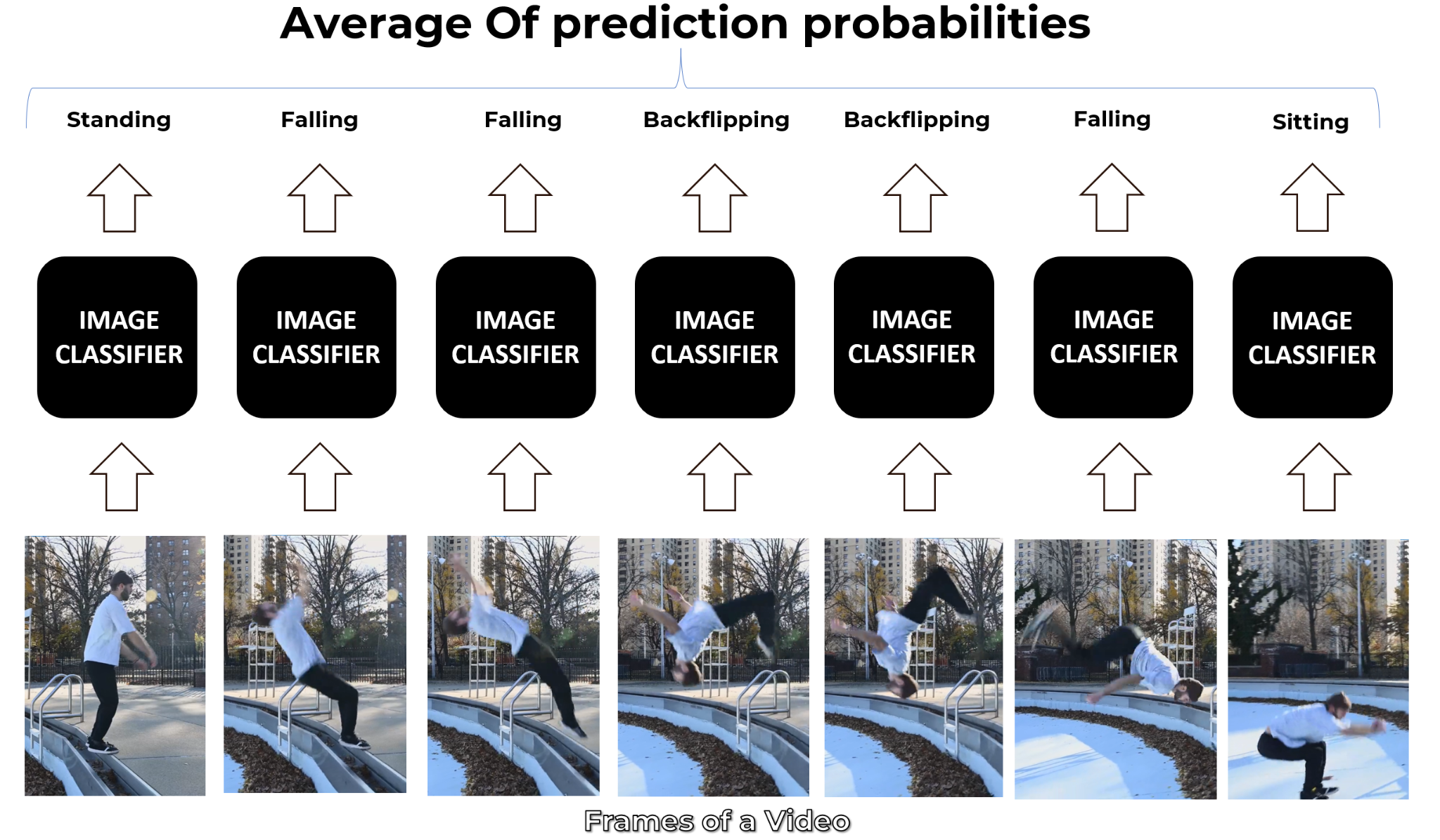


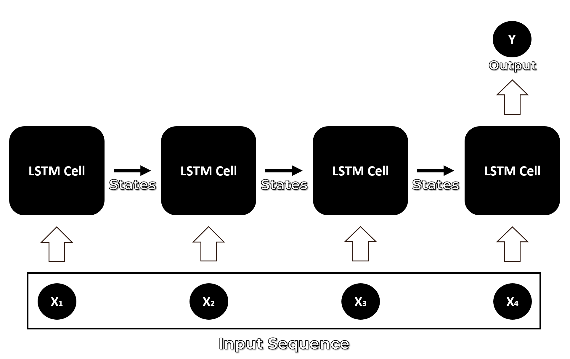

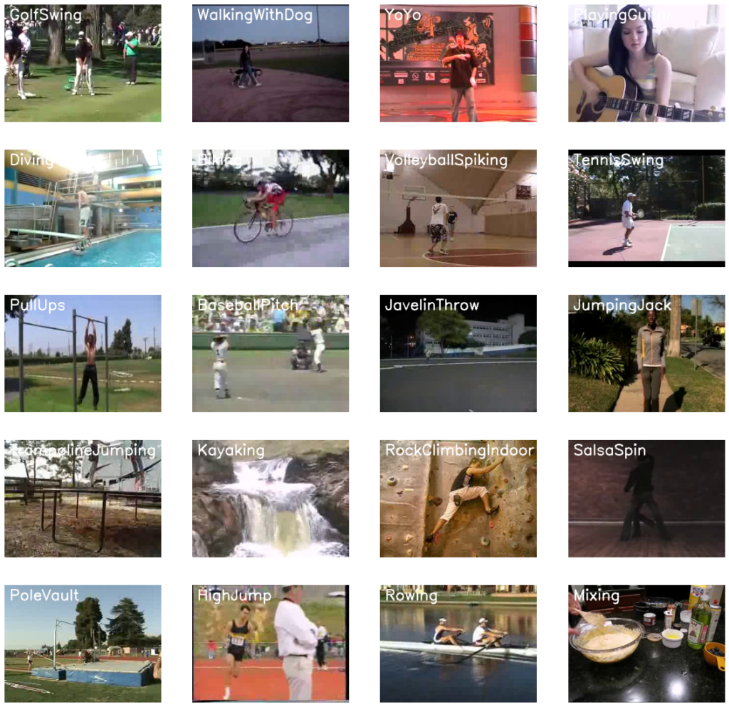
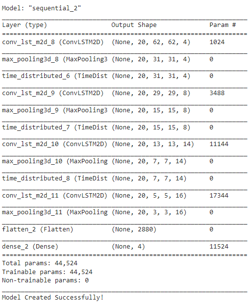
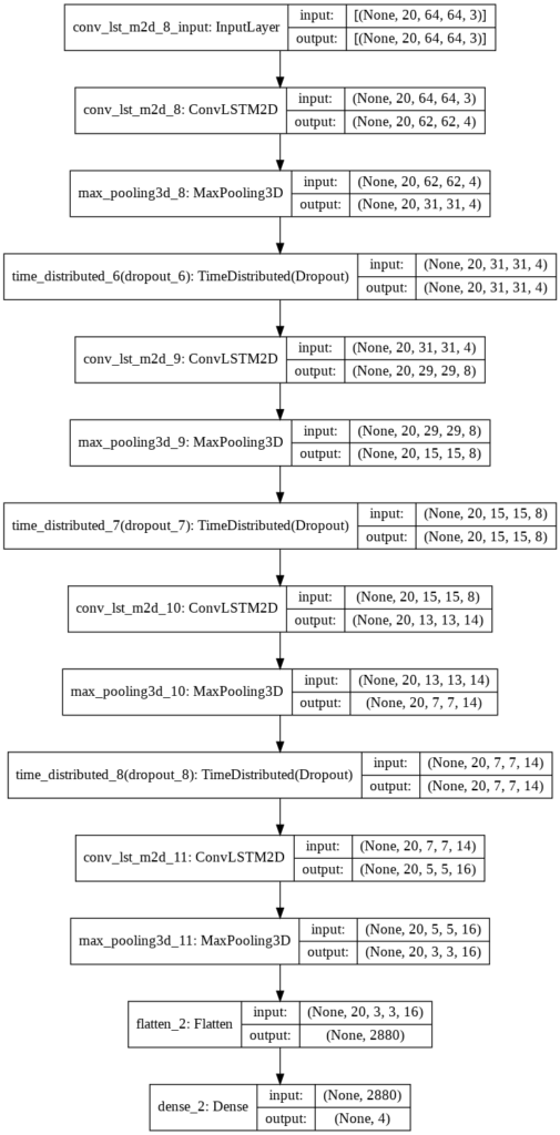
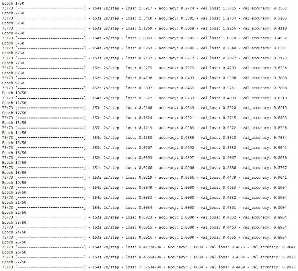
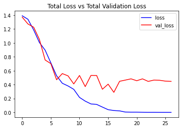
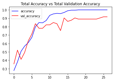
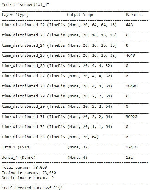
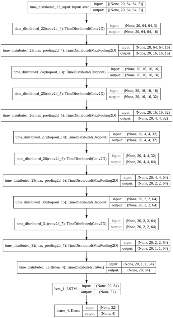
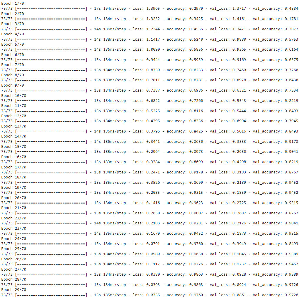
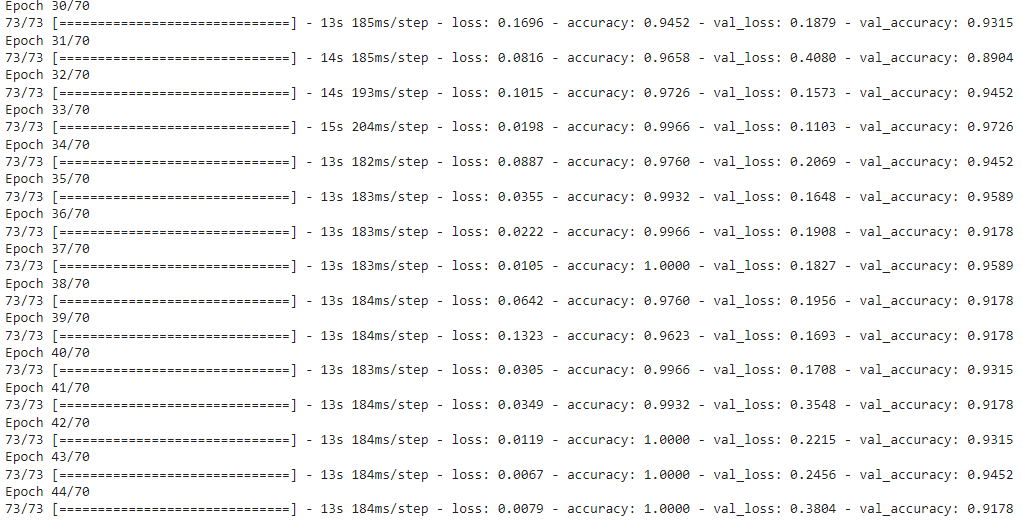
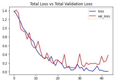
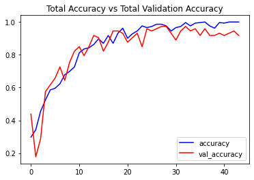


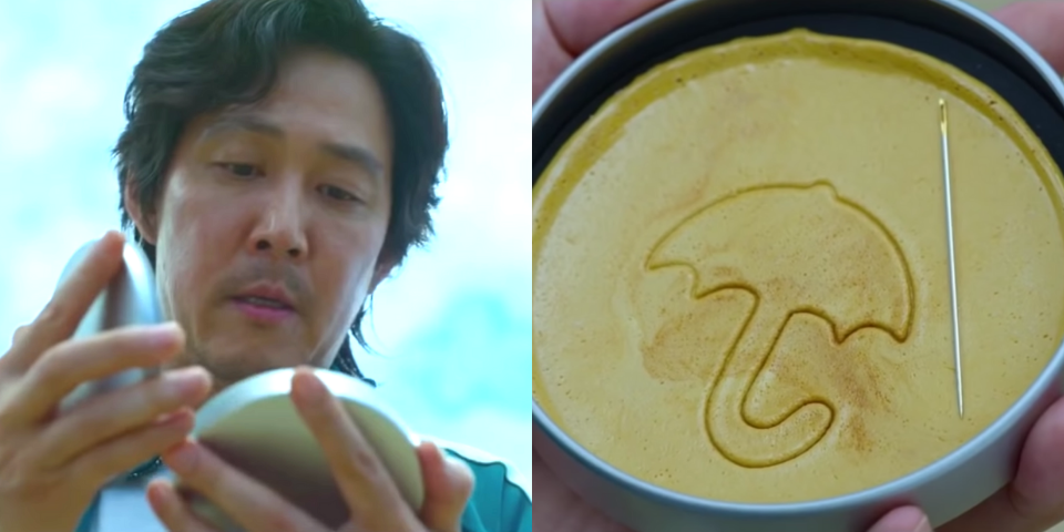


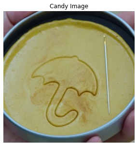


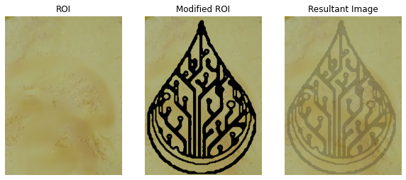
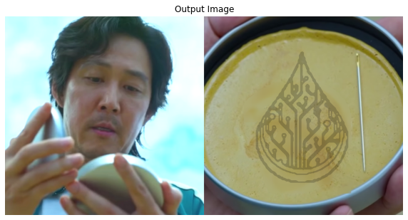


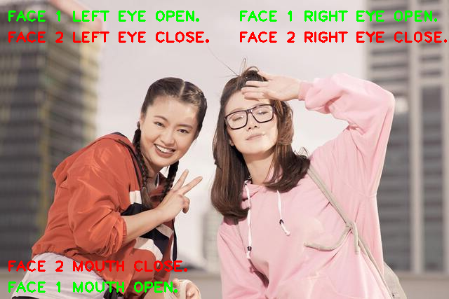
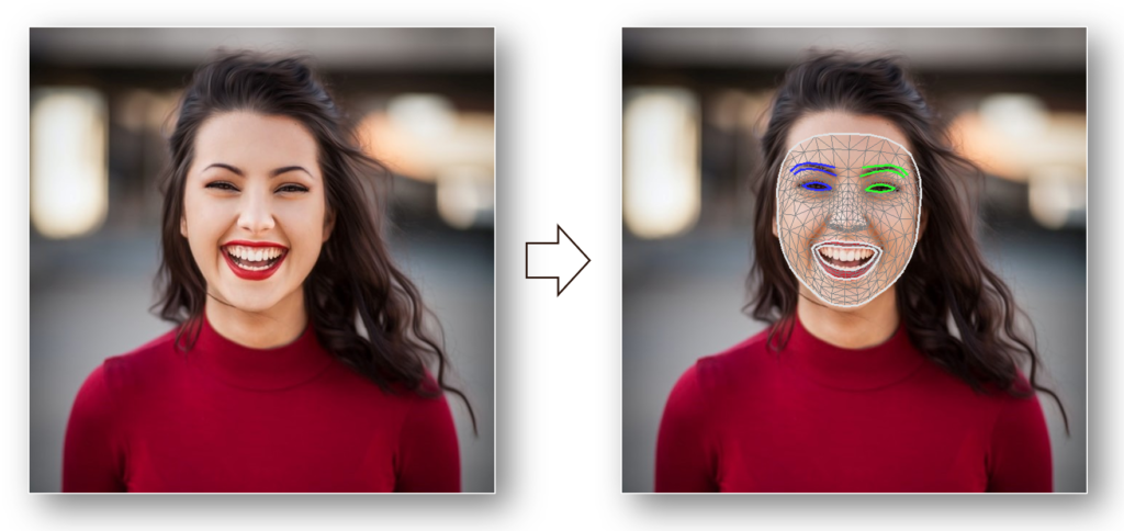


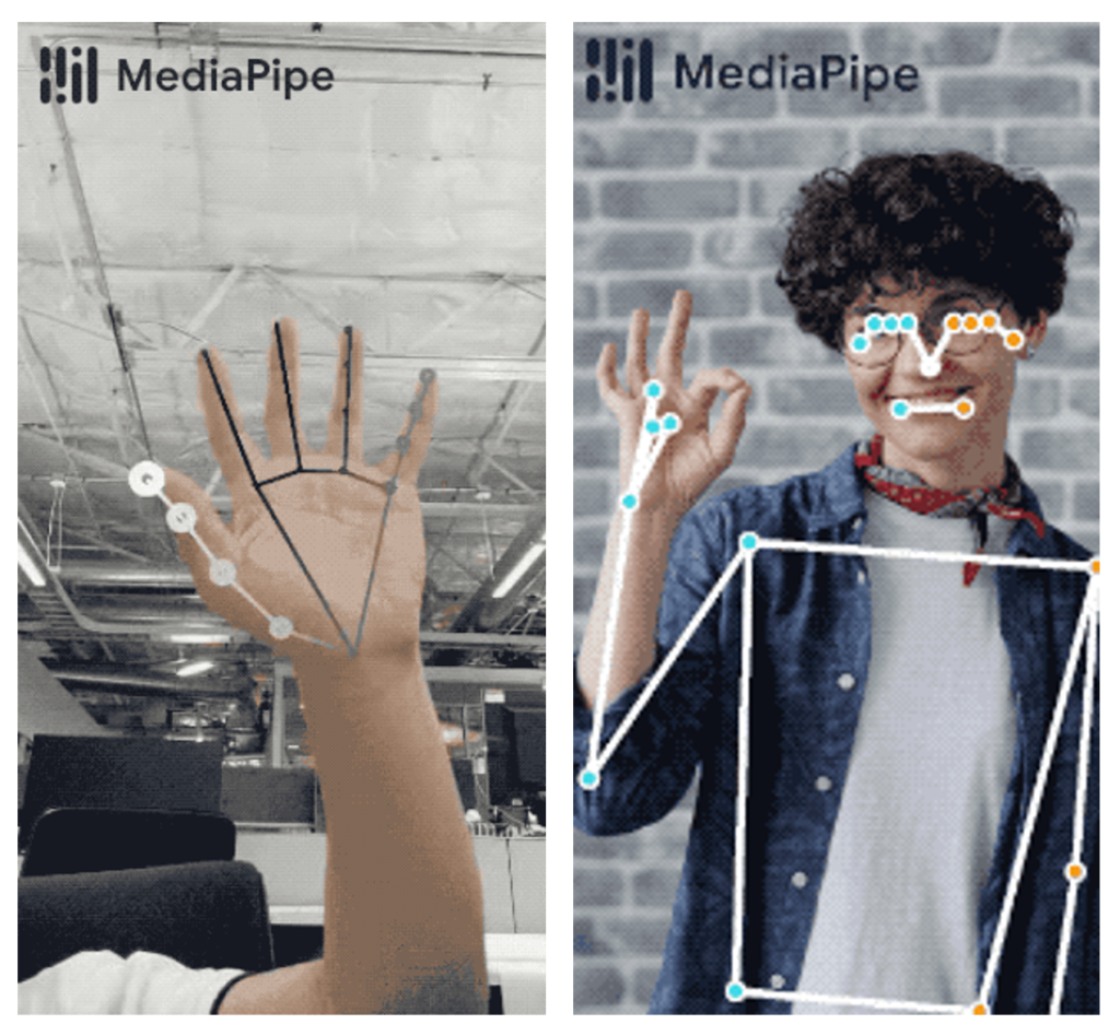

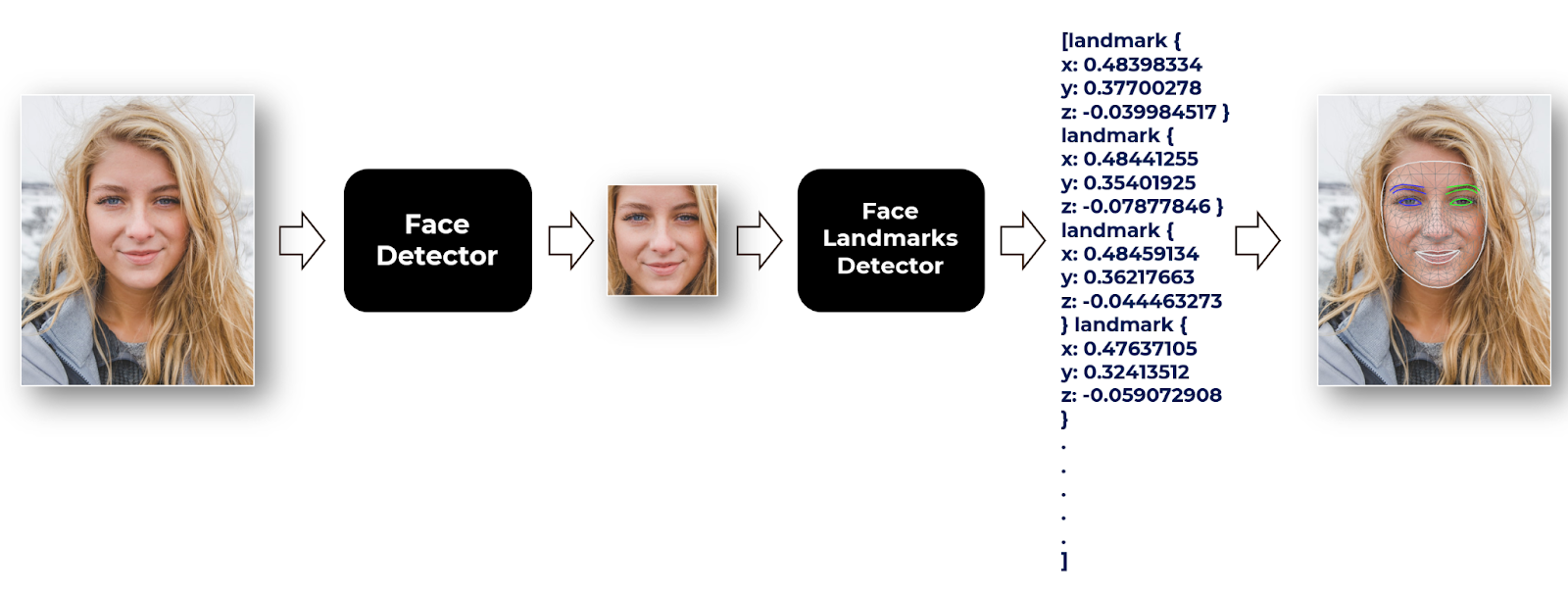

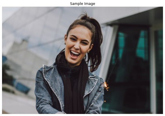

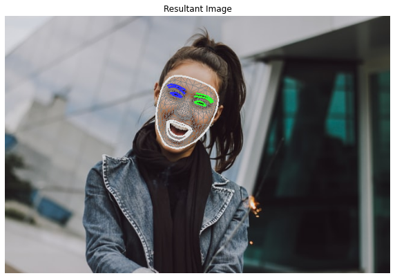

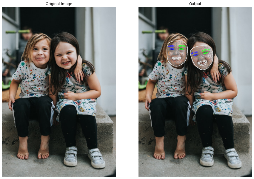


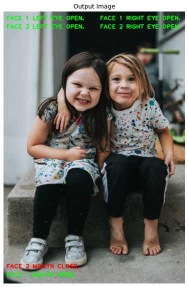
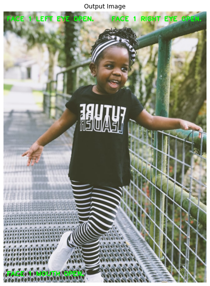


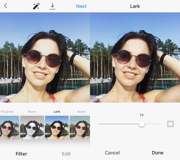

